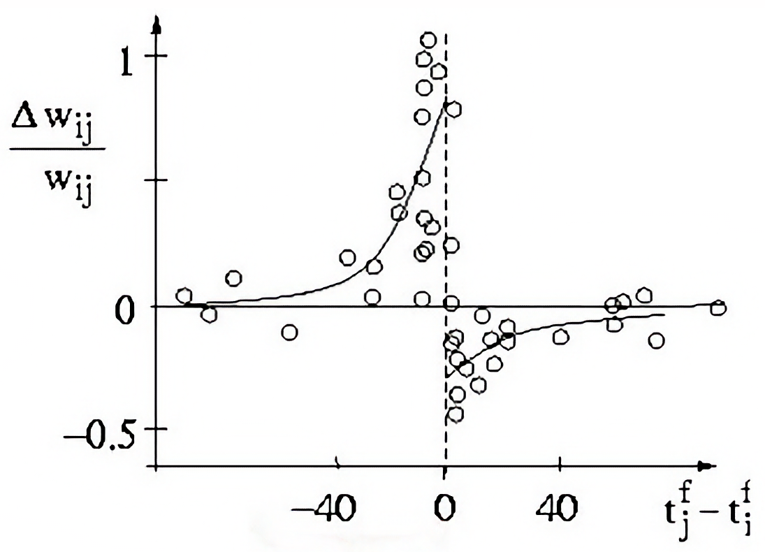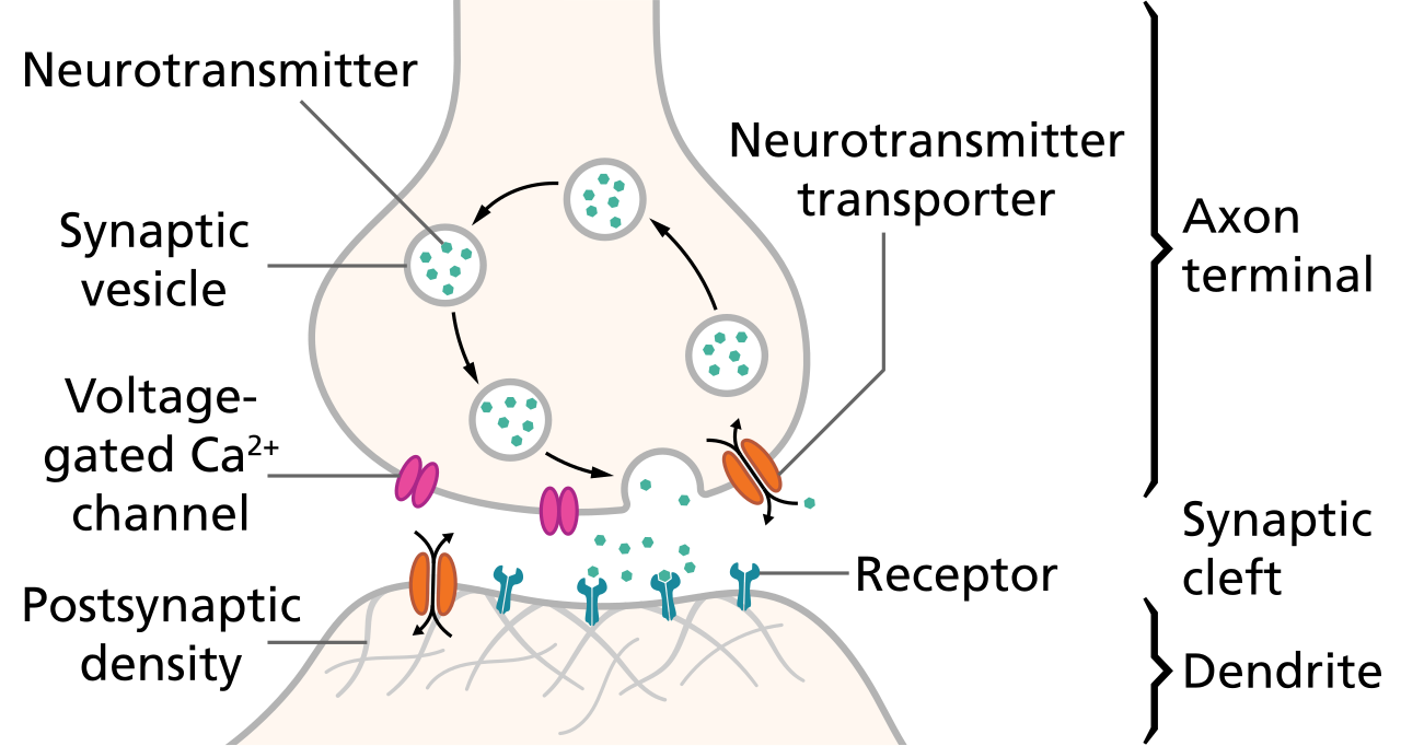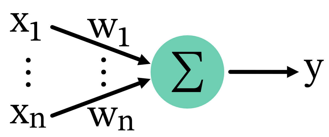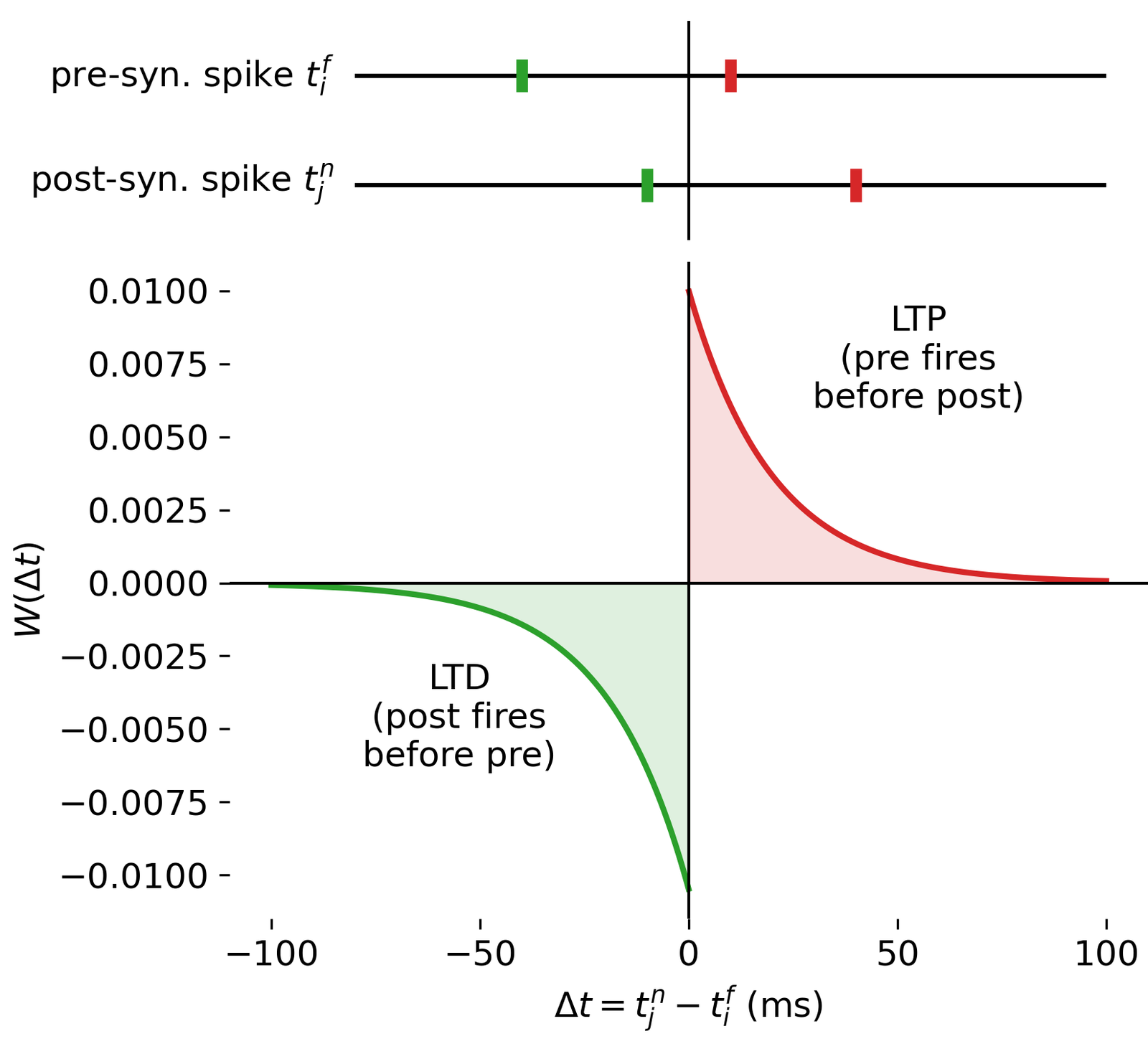
<?xml version="1.0" encoding="utf-8"?><feed xmlns="http://www.w3.org/2005/Atom" ><generator uri="https://jekyllrb.com/" version="4.4.1">Jekyll</generator><link href="/feed.xml" rel="self" type="application/atom+xml" /><link href="/" rel="alternate" type="text/html" /><updated>2026-05-25T01:03:03+02:00</updated><id>/feed.xml</id><title type="html">Fabrizio Musacchio</title><subtitle>I want to understand how the brain works. My research interests lie at the intersection of neuroscience, behavioral science and computational neuroscience. I’m especially interested in how the brain learns and which processes drive learning.</subtitle><author><name>{&quot;name&quot;=&gt;nil, &quot;avatar&quot;=&gt;&quot;/assets/images/profile.jpg&quot;, &quot;bio&quot;=&gt;&quot;&quot;, &quot;location&quot;=&gt;nil, &quot;links&quot;=&gt;[{&quot;label&quot;=&gt;&quot;Cologne, Germany&quot;, &quot;icon&quot;=&gt;&quot;fas fa-map-marker&quot;, &quot;url&quot;=&gt;&quot;https://goo.gl/maps/LZgMvTkEDgAZXSVaA&quot;}, {&quot;label&quot;=&gt;&quot;Postdoc at the DZNE Research Center&quot;, &quot;icon&quot;=&gt;&quot;fas fa-university&quot;, &quot;url&quot;=&gt;&quot;https://www.dzne.de/en/research/research-areas/fundamental-research/research-groups/fuhrmann/research-areasfocus/&quot;}, {&quot;label&quot;=&gt;&quot;Contact&quot;, &quot;icon&quot;=&gt;&quot;far fa-envelope&quot;, &quot;url&quot;=&gt;&quot;/contact&quot;}, {&quot;label&quot;=&gt;&quot;GitHub&quot;, &quot;icon&quot;=&gt;&quot;fab fa-github&quot;, &quot;url&quot;=&gt;&quot;https://github.com/fabriziomusacchio&quot;}, {&quot;label&quot;=&gt;&quot;Google Scholar&quot;, &quot;icon&quot;=&gt;&quot;fas fa-graduation-cap&quot;, &quot;url&quot;=&gt;&quot;https://scholar.google.com/citations?user=zb_0liUAAAAJ&amp;hl=de&quot;}, {&quot;label&quot;=&gt;&quot;ORCID&quot;, &quot;icon&quot;=&gt;&quot;fab fa-orcid&quot;, &quot;url&quot;=&gt;&quot;https://orcid.org/0000-0002-9043-3349&quot;}, {&quot;label&quot;=&gt;&quot;ResearchGate&quot;, &quot;icon&quot;=&gt;&quot;fab fa-researchgate&quot;, &quot;url&quot;=&gt;&quot;https://www.researchgate.net/profile/Fabrizio-Musacchio&quot;}, {&quot;label&quot;=&gt;&quot;Twitter&quot;, &quot;icon&quot;=&gt;&quot;fab fa-twitter&quot;, &quot;url&quot;=&gt;&quot;https://twitter.com/FabMusacchio&quot;}, {&quot;label&quot;=&gt;&quot;Mastodon&quot;, &quot;icon&quot;=&gt;&quot;fab fa-mastodon&quot;, &quot;url&quot;=&gt;&quot;https://sigmoid.social/@pixeltracker&quot;}, {&quot;label&quot;=&gt;&quot;Flickr&quot;, &quot;icon&quot;=&gt;&quot;fab fa-flickr&quot;, &quot;url&quot;=&gt;&quot;https://flickr.com/photos/fabriziomusacchio/&quot;}]}</name></author><entry><title type="html">Virchow’s Cellularpathologie: A foundational work in the history of medicine and neuroscience</title><link href="/blog/2026-05-14-virchow_cellularpathologie/" rel="alternate" type="text/html" title="Virchow’s Cellularpathologie: A foundational work in the history of medicine and neuroscience" /><published>2026-05-14T13:57:00+02:00</published><updated>2026-05-14T13:57:00+02:00</updated><id>/blog/virchow_cellularpathologie</id><content type="html" xml:base="/blog/2026-05-14-virchow_cellularpathologie/"><![CDATA[<p>After that <a href="/blog/2026-05-09-helmholtz_dissertation/">talk by Kettenmann</a>, I could not quite let go of the remaining historical connections that he had mentioned. One of them was the fact that Rudolf Virchow, the founder of cellular pathology, had introduced the distinction between neurons and glial cells in the mid 1850s. And this distinction, as Kettenmann emphasized, was crucial for the later development of <a href="/blog/2026-02-04-neural_dynamics/">neuroscience</a>, because it provided the conceptual framework for understanding the cellular composition of the nervous system.</p>

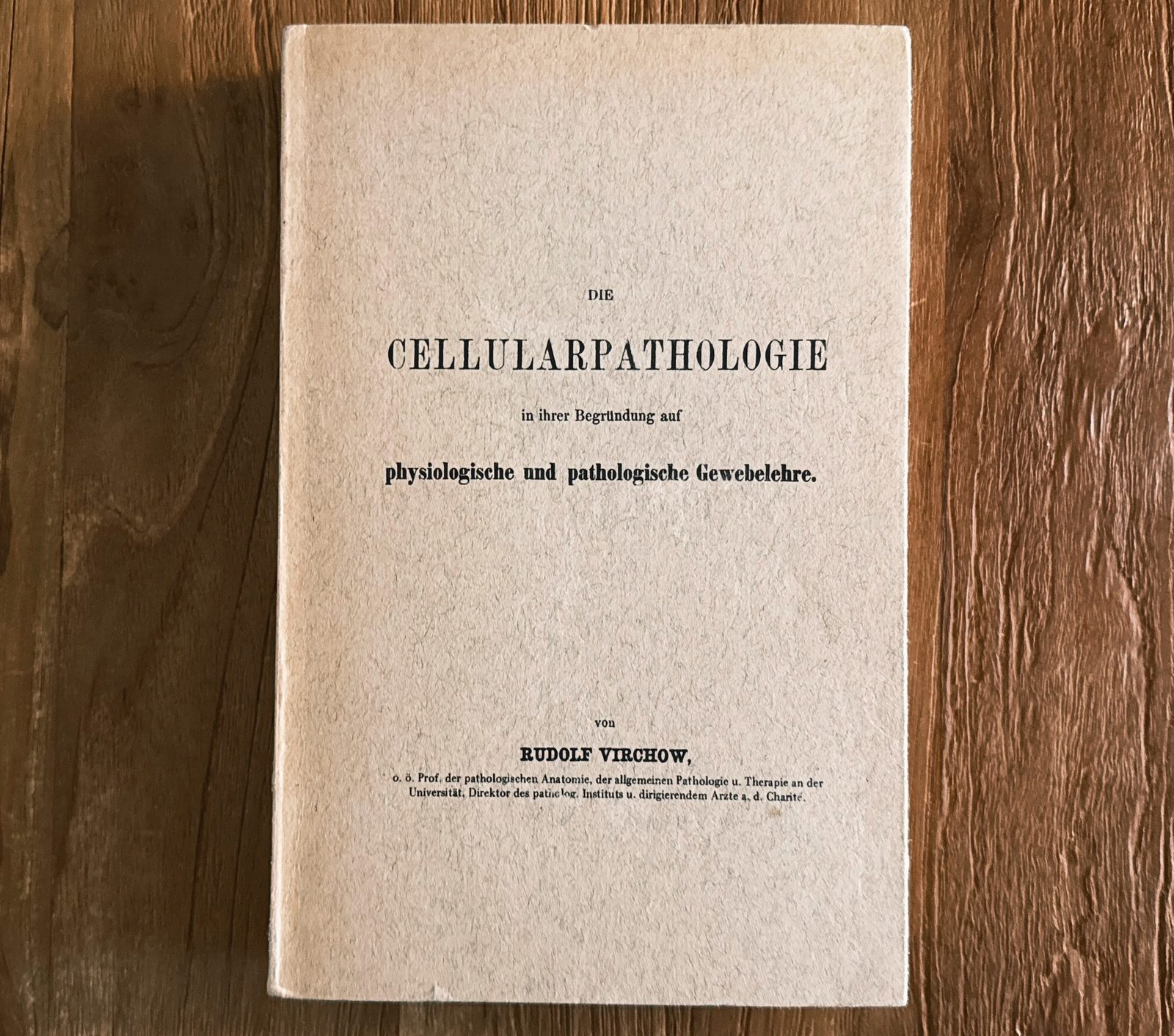
<p class="align-caption"><a href="https://assets.fmusacchio.com/assets/posts/neuroscience/virchow_cellularpathologie_cover_1600px.jpg" title="The cover of my personal copy of Virchow's Cellularpathologie, which I ordered from a second-hand book store."><img src="https://assets.fmusacchio.com/assets/posts/neuroscience/virchow_cellularpathologie_cover_800px.jpg" width="100%" alt="The cover of my personal copy of Virchow's Cellularpathologie, which I ordered from a second-hand book store." /></a><br />
The cover of my personal copy of Virchow’s <em>Cellularpathologie</em>, which I ordered from a second-hand book store. The book is in German, but there may be English translations available as well.</p>

<p>I could not resist buying a physical copy of Virchow’s <em>Cellularpathologie</em>. A used reproduction from 1956, nothing special. But it felt oddly appropriate. As someone still relatively new to neuroscience, I did not know this work before. However, as a side note, I had already encountered Virchow’s name almost on a daily basis: In the city where I grew up, I lived in a neighbourhood where almost all streets were named after German scientists. One of them was <em>Virchowstraße</em><sup id="fnref:2"><a href="#fn:2" class="footnote" rel="footnote" role="doc-noteref">1</a></sup> (<em>Virchow Street</em>), which I passed by every day on my way to school. Of course, I knew what Virchow was famous for, but I had never read any of his work.</p>

<p class="align-caption"><a href="https://assets.fmusacchio.com/assets/posts/neuroscience/virchow_cellularpathologie_cover_2_1600px.jpg" title="Zoom onto the cover of Virchow's Cellularpathologie."><img src="https://assets.fmusacchio.com/assets/posts/neuroscience/virchow_cellularpathologie_cover_2_800px.jpg" width="100%" alt="Zoom onto the cover of Virchow's Cellularpathologie." /></a><br />
Zoom onto the cover of Virchow’s <em>Cellularpathologie</em> (my personal copy).</p>

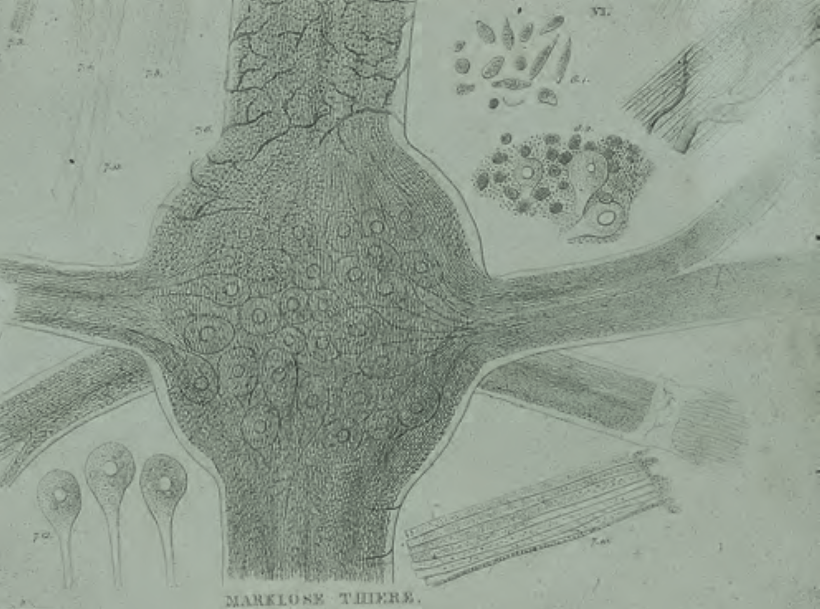
<p>I did not read the entire book, since it is quite long and dense, and, from a physicist’s perspective, several chapters are out of my depth. However, since it was written in German, it was of course no problem to understand the text. I found it fascinating how structured and precise this early scientific work is. It felt almost like reading a modern scientific book. Of course, the figures were not made with modern software, as we would do today. Instead, <a href="/weekend_stories/told/2024/2024-08-09-ukiyo_e/">woodcut illustrations</a> were used, which achieve such a high level of detail and clarity that they even surpass some modern illustrations in my view. The book is organized into 20 lectures, each focused on a specific aspect, and the arguments are built step by step, with careful attention to evidence and logical structure.</p>

<p>In this post, I want to share some of the insights I gained from engaging with Virchow’s <em>Cellularpathologie</em>. I will not attempt to summarize the entire book, but rather focus on some key themes and implications that I found interesting.</p>

<h2 id="virchow-and-the-conceptual-shift-in-medicine">Virchow and the conceptual shift in medicine</h2>
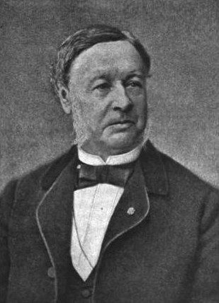
<p>Rudolf Virchow (1821–1902) is often regarded as one of the most influential figures in the history of medicine. He was a physician, pathologist, anthropologist, politician, and social reformer, and his work fundamentally changed how disease was understood in the 19th century. Today, Virchow is primarily remembered as the founder of cellular pathology, but his scientific influence extended much further. He contributed to histology, pathology, epidemiology, and public health, argued strongly for the social dimension of medicine, and introduced or popularized concepts and terms that remain central to medicine today, including thrombosis, embolism, leukemia, and neuroglia.</p>

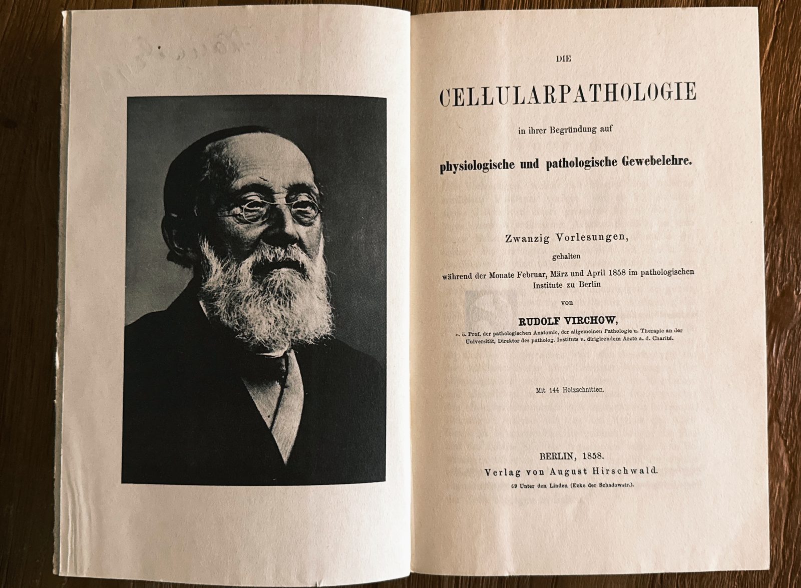
<p class="align-caption"><a href="https://assets.fmusacchio.com/assets/posts/neuroscience/virchow_cellularpathologie_virchow_1600px.jpg" title="First pages of Virchow's Cellularpathologie, with a photograph of Virchow himself on the left."><img src="https://assets.fmusacchio.com/assets/posts/neuroscience/virchow_cellularpathologie_virchow_800px.jpg" width="100%" alt="First pages of Virchow's Cellularpathologie, with a photograph of Virchow himself on the left." /></a><br />
First pages of Virchow’s <em>Cellularpathologie</em>, with a photograph of Virchow himself on the left. Source: Reproduced from Rudolf Virchow, <em>Die Cellularpathologie in ihrer Begründung auf physiologische und pathologische Gewebelehre</em>, 1858. Photograph of the printed figure taken by myself. Original work in the public domain.</p>

<p>His most influential work, however, was undoubtedly <em>Cellularpathologie</em>, first published in 1858. The book laid the conceptual foundation for modern pathology and had profound implications for how disease itself was understood.</p>

<p>Virchow’s central idea is often summarized in a single statement:</p>

<blockquote>
  <p>Omnis cellula e cellula</p>

  <p>Every cell arises from another cell.</p>
</blockquote>

<p>At first glance, this sounds almost trivial from a modern perspective. However, in the mid 19th century, this statement directly contradicted older ideas about spontaneous generation and the formation of tissues from amorphous substances. It established continuity at the cellular level as the fundamental principle of life. More importantly, Virchow extended this principle from physiology to pathology. Disease, in his view, is not a disturbance of abstract bodily “fluids” or humors such as blood, phlegm, black bile, and yellow bile, as in ancient medicine, but a disturbance of cells. This is the conceptual core of cellular pathology.</p>

<p>This insight has profound implications: If every physiological process is rooted in cellular processes, then every pathological process must also be reducible to changes in cellular structure, function, or proliferation. In modern terms, this marks a shift from descriptive medicine at the level of organs and symptoms toward a mechanistic and microscopic understanding of disease.</p>

<h2 id="the-lectures">The lectures</h2>
<p>Virchow’s <em>Cellularpathologie</em> is not a monolithic treatise in the traditional sense. It is a collection of 20 lectures, delivered in early 1858 at the Pathological Institute in Berlin and later transcribed and edited for publication. This also explains the style of the work: It is didactic, structured around demonstrations, and closely tied to visual material such as microscopic preparations and woodcut illustrations.</p>

<p class="align-caption"><a href="https://assets.fmusacchio.com/assets/posts/neuroscience/virchow_cellularpathologie_lecture_1_1600px.jpg" title="Cover of the first lecture of Virchow's Cellularpathologie."><img src="https://assets.fmusacchio.com/assets/posts/neuroscience/virchow_cellularpathologie_lecture_1_800px.jpg" width="100%" alt="Cover of the first lecture of Virchow's Cellularpathologie." /></a><br />
Cover of the first lecture of Virchow’s <em>Cellularpathologie</em>. Source: Woodcut illustration reproduced from Rudolf Virchow, <em>Die Cellularpathologie in ihrer Begründung auf physiologische und pathologische Gewebelehre</em>, 1858. Photograph of the printed figure taken by myself. Original work in the public domain.</p>

<p>The work begins with a systematic overview of cell theory, integrating botanical and zoological observations. The inclusion of plant cells alongside animal tissues reflects the universality of the cellular principle. The same structural logic applies across living systems, whether in plant tissue, cartilage, liver, or nervous tissue, as illustrated in the early figures of the book.</p>

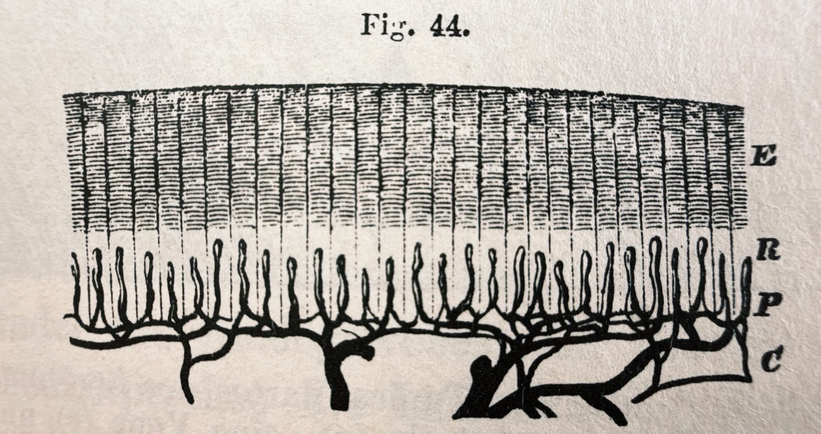
<p class="align-caption"><a href="https://assets.fmusacchio.com/assets/posts/neuroscience/virchow_cellularpathologie_fig44_1600px.jpg" title="Woodcut illustration of an injection preparation of the skin, vertical cut."><img src="https://assets.fmusacchio.com/assets/posts/neuroscience/virchow_cellularpathologie_fig44_800px.jpg" width="100%" alt="Woodcut illustration of an injection preparation of the skin, vertical cut." /></a><br />
Woodcut illustration of an injection preparation of the skin, vertical cut. E: Epidermis, R: Rete Malpighii, P: Papilla with its up and down projecting vessels, C: Cutis. Source: Woodcut illustration (Fig. 44) reproduced from Rudolf Virchow, <em>Die Cellularpathologie in ihrer Begründung auf physiologische und pathologische Gewebelehre</em>, 1858. Photograph of the printed figure taken by myself. Original work in the public domain.</p>

<p>From this foundation, Virchow gradually develops the framework of cellular pathology in detail. Much of the book can be understood as a systematic attempt to establish the cell as the central explanatory unit of medicine.</p>

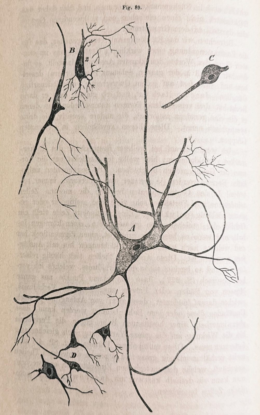
<p class="align-caption"><a href="https://assets.fmusacchio.com/assets/posts/neuroscience/virchow_cellularpathologie_fig89_1600px.jpg" title="Woodcut illustration of Ganglion cells from the central organs."><img src="https://assets.fmusacchio.com/assets/posts/neuroscience/virchow_cellularpathologie_fig89_800px.jpg" width="100%" alt="Woodcut illustration of Ganglion cells from the central organs." /></a><br />
Woodcut illustration of Ganglion cells from the central organs: A, B, C from the spinal cord, based on preparations by Mr. Gerlach; D from the cerebral cortex. A: Large, multi-dendritic (multipolar, polyclonal) cells from the anterior horns (motor cells). B: Smaller cells with 3 larger processes from the posterior horns (sensory cells). C: Two-branched (bipolar, diclonal), more rounded cells from the vicinity of the posterior commissure (sympathetic cells). Magnification: 300. Source: Woodcut illustration (Fig. 89) reproduced from Rudolf Virchow, <em>Die Cellularpathologie in ihrer Begründung auf physiologische und pathologische Gewebelehre</em>, 1858. Photograph of the printed figure taken by myself. Original work in the public domain.</p>

<p>In the lectures, Virchow explicitly argues against older humoral and organ-centered views of disease and instead localizes pathological processes at the cellular level. However, what is particularly interesting here is how concretely he develops this argument. Rather than presenting a purely abstract theory, he continuously moves between microscopic observations, tissue morphology, pathological examples, and conceptual interpretation.</p>

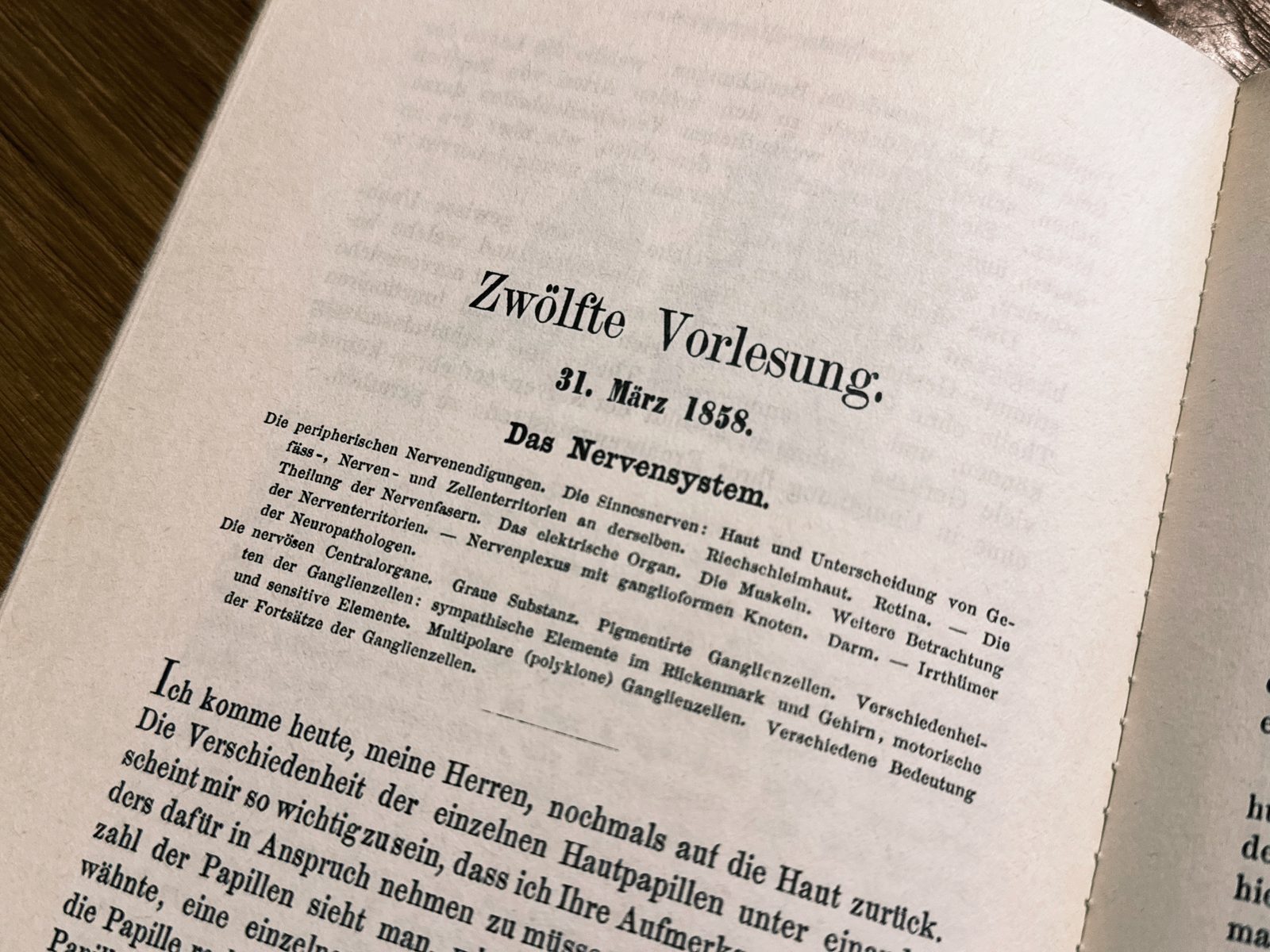
<p class="align-caption"><a href="https://assets.fmusacchio.com/assets/posts/neuroscience/virchow_cellularpathologie_lecture_12_1600px.jpg" title="Cover of the 12th lecture of Virchow's *Cellularpathologie*, focused on the nervous system."><img src="https://assets.fmusacchio.com/assets/posts/neuroscience/virchow_cellularpathologie_lecture_12_800px.jpg" width="100%" alt="Cover of the 12th lecture of Virchow's *Cellularpathologie*, focused on the nervous system." /></a><br />
Cover of the 12th lecture of Virchow’s <em>Cellularpathologie</em>, which is focused on the nervous system. Source: Woodcut illustration reproduced from Rudolf Virchow, <em>Die Cellularpathologie in ihrer Begründung auf physiologische und pathologische Gewebelehre</em>, 1858. Photograph of the printed figure taken by myself. Original work in the public domain.</p>

<p>Similarly, Virchow repeatedly emphasizes that pathological processes are not fundamentally separate from physiological ones. Disease is not treated as something metaphysically distinct from normal life processes, but as an alteration, dysregulation, or exaggeration of normal cellular activity. In his lectures, he establishes this view not only philosophically, but through numerous examples involving growth, degeneration, inflammation, and tissue remodeling. The detailed discussion of inflammation is especially interesting here: Inflammation is no longer described merely through externally visible symptoms such as heat, redness, and swelling, but as a sequence of cellular events involving the accumulation, transformation, and activity of specific cells. Likewise, tumors are interpreted not as foreign entities or parasitic growths, but as the result of abnormal cellular proliferation originating from the body’s own tissues.</p>

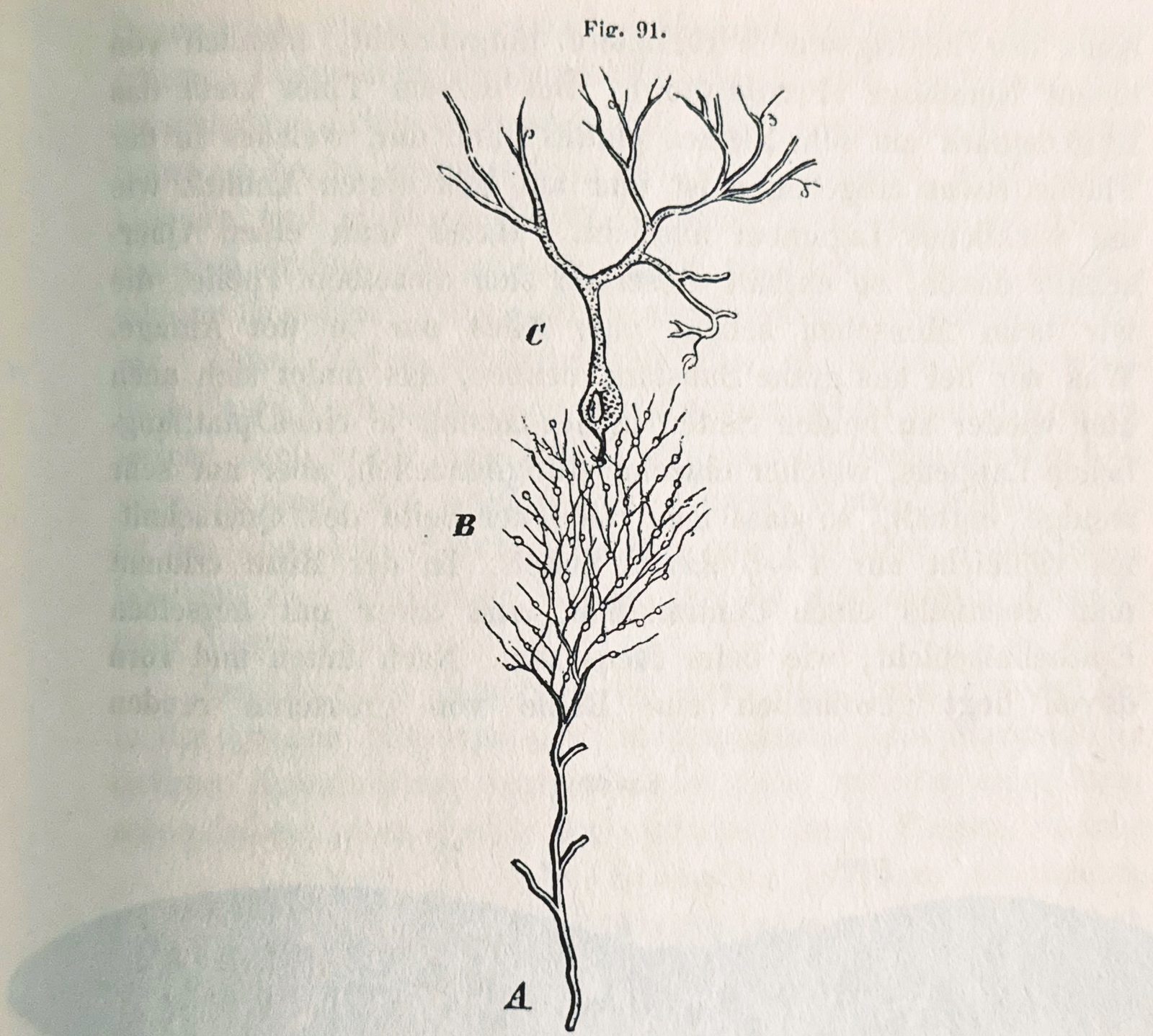
<p>And Virchow reinforces his arguments with an, at that time, extensive use of microscopic images, which range from plant cells to cartilage, liver cells, capillaries, ganglion cells, and pathological tissues:</p>

<p class="align-caption"><a href="https://assets.fmusacchio.com/assets/posts/neuroscience/virchow_cellularpathologie_fig91_1600px.jpg" title="Schematic representation of nerve fiber patterns in the cerebellar cortex according to Gerlach."><img src="https://assets.fmusacchio.com/assets/posts/neuroscience/virchow_cellularpathologie_fig91_800px.jpg" width="100%" alt="Schematic representation of nerve fiber patterns in the cerebellar cortex according to Gerlach." /></a><br />
Schematic representation of nerve fiber patterns in the cerebellar cortex according to Gerlach. (Microscopic Studies, Plate I, Fig. 3.) A: white matter; B, C: gray matter; B: granular layer; C: cell layer. Source: Woodcut illustration (Fig. 91) reproduced from Rudolf Virchow, <em>Die Cellularpathologie in ihrer Begründung auf physiologische und pathologische Gewebelehre</em>, 1858. Photograph of the printed figure taken by myself. Original work in the public domain.</p>

<p>Another important aspect is Virchow’s insistence on continuity. There is no abrupt transition from health to disease at the level of fundamental principles. Instead, there exists a continuous spectrum of cellular states and transformations. This idea feels remarkably modern, since many diseases today are understood not as entirely separate biological phenomena, but as dysregulated versions of normal cellular processes.</p>

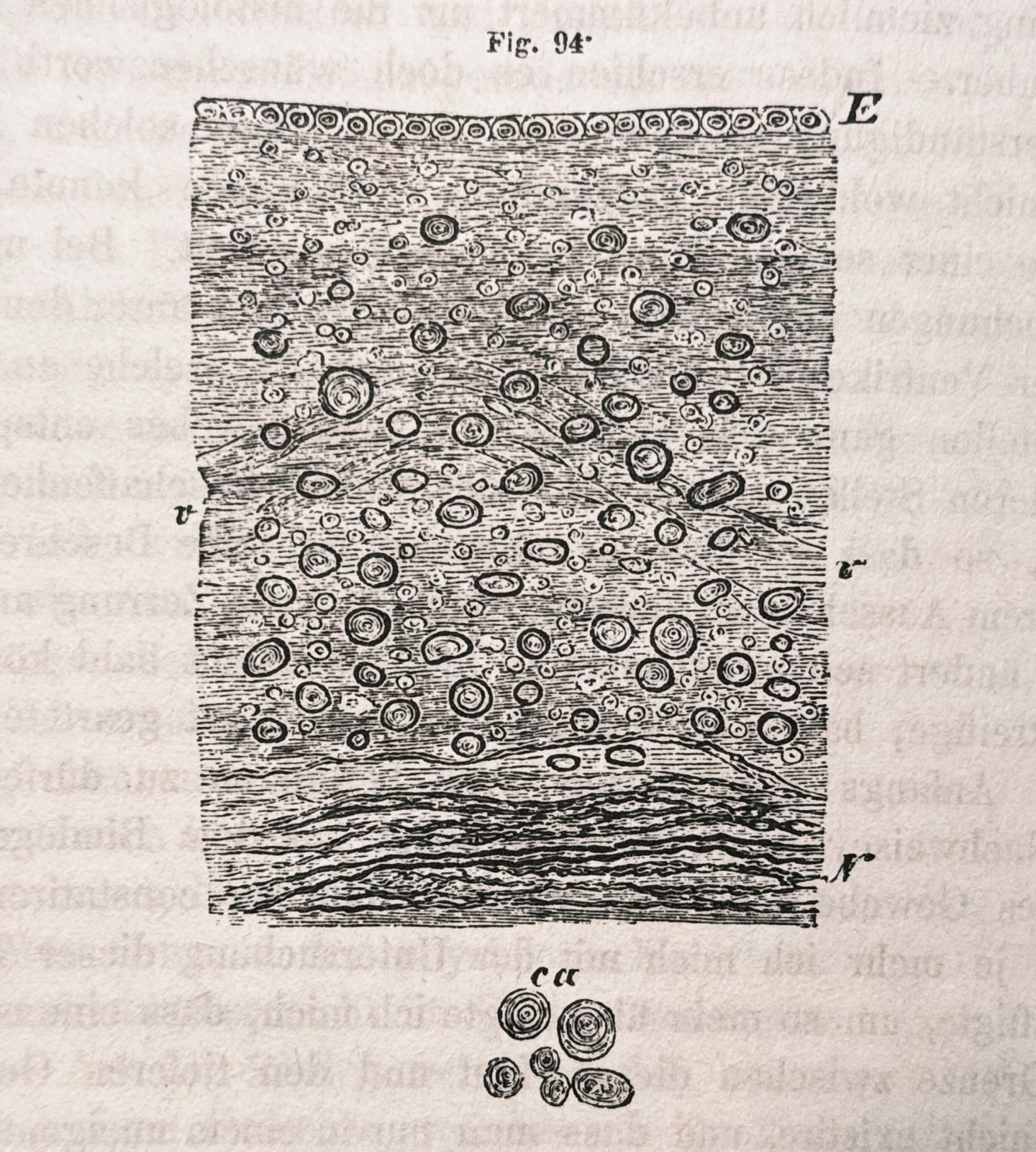
<p>Finally, and in direct connection to our <a href="/blog/2026-05-09-helmholtz_dissertation/">earlier discussion of Helmholtz</a>, Virchow introduced the concept of neuroglia as a distinct cellular component of nervous tissue. This distinction between neurons and glial cells provided an important conceptual framework for later <a href="/blog/2026-02-04-neural_dynamics/">neuroscience</a> and fundamentally changed how the nervous system was understood at the cellular level. What Virchow recognized was that the nervous system could not be reduced to nerve fibers and nerve cells alone. It also contained another cellular and structural component, which he interpreted as a kind of connective or supporting tissue of the nervous system. The term <em>neuroglia</em> itself expresses this idea: A “nerve glue”, a tissue that holds the nervous elements together:</p>

<p class="align-caption"><a href="https://assets.fmusacchio.com/assets/posts/neuroscience/virchow_cellularpathologie_fig94_1600px.jpg" title="Woodcut illustration of the ependyma of the ventricles and neuroglia from the floor of the fourth ventricle."><img src="https://assets.fmusacchio.com/assets/posts/neuroscience/virchow_cellularpathologie_fig94_800px.jpg" width="100%" alt="Woodcut illustration of the ependyma of the ventricles and neuroglia from the floor of the fourth ventricle." /></a><br />
Woodcut illustration of the ependyma of the ventricles and neuroglia from the floor of the fourth ventricle. E: epithelium, N: nerve fibers. In between lies the free portion of the neuroglia, containing numerous connective tissue cells and nuclei; at v is a blood vessel; elsewhere, numerous corpora amylacea are visible, which are shown in isolation at ca. Magnification: 300. Source: Woodcut illustration (Fig. 94) reproduced from Rudolf Virchow, <em>Die Cellularpathologie in ihrer Begründung auf physiologische und pathologische Gewebelehre</em>, 1858. Photograph of the printed figure taken by myself. Original work in the public domain.</p>

<p>From a modern perspective, this interpretation was still limited, because glial cells are no longer understood as merely passive support elements. <a href="/blog/2025-06-29-astrocyte_enhance_plasticity/">Astrocytes</a>, oligodendrocytes, <a href="/research/2025_motila">microglia</a>, and other glial cell types are now known to participate actively in homeostasis, metabolism, myelination, immune defense, synaptic regulation, and <a href="/research/2026_microglia_glioblastoma_crosstalk">disease processes</a>. But Virchow’s conceptual step was nevertheless crucial: He separated the nervous system into more than one cellular category and thereby opened the possibility of asking what these non-neuronal cells are, where they come from, and what they do.</p>

<h2 id="conceptual-implications">Conceptual implications</h2>
<p>What I take away from researching and reading Virchow’s <em>Cellularpathologie</em> is that it represents a major conceptual shift in the history of medicine. It is not just a collection of observations or a description of pathological phenomena. It is an attempt to reorganize the entire field of medicine around the cell as the fundamental unit of life and disease. Virchow constructs a coherent explanatory framework that connects anatomy, physiology, pathology, microscopy, and tissue structure into a unified view of disease. In this sense, the book can be regarded as on of the scientifically most important works in the history of medicine, and it laid the groundwork for many subsequent developments in pathology, histology, and <a href="/blog/2026-02-04-neural_dynamics/">neuroscience</a>.</p>

<p>Several aspects of Virchow’s reasoning still feel surprisingly familiar, at least from what I can recognize as a non-medical reader. The idea that disease emerges from altered cellular states, that pathological and physiological processes are deeply connected, and that microscopic structures can provide mechanistic explanations for macroscopic symptoms remains central to biomedical science today.</p>

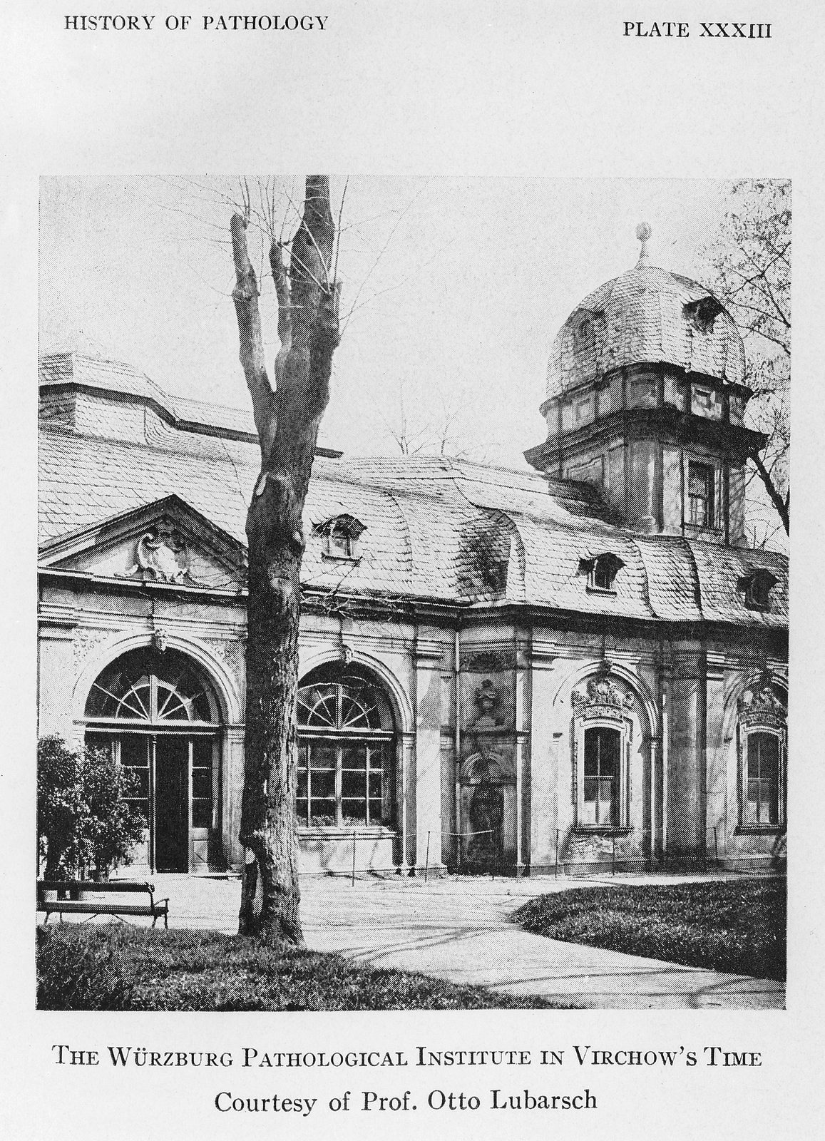
<p class="align-caption"><a href="https://assets.fmusacchio.com/assets/posts/neuroscience/Pathological_institution,_Wurzburg_in_Virchow's_time_Wellcome_M0017265_1600px.jpg" title="The garden pavilion of the Juliusspital in Würzburg housed Virchow's Institute of Pathology until 1853."><img src="https://assets.fmusacchio.com/assets/posts/neuroscience/Pathological_institution,_Wurzburg_in_Virchow's_time_Wellcome_M0017265_800px.jpg" width="100%" alt="The garden pavilion of the Juliusspital in Würzburg housed Virchow's Institute of Pathology until 1853." /></a><br />
The garden pavilion of the Juliusspital in Würzburg housed Virchow’s Institute of Pathology until 1853. Source: <a href="https://w.wiki/NJsm">Wikimedia Commons</a><span style="color:#d5d6db;font-size:0.8rem;">ꜛ</span> (license: CC BY-SA 4.0).</p>

<p>Engaging with Virchow after reading <a href="/blog/2026-05-09-helmholtz_dissertation/">Helmholtz’s dissertation</a> also highlights an interesting historical contrast. Helmholtz’s dissertation is to some extent a bit more observational and comparative. Virchow, by contrast, is much more focused on conceptual integration and theoretical organization. He builds a framework in which such structures acquire general pathological meaning. In this sense, the two works together provide an interesting glimpse into the emergence of modern life sciences during the 19th century, which could, in a very simplified way, be seen as: One focused on observation and comparative anatomy, the other on conceptual unification and medical interpretation.</p>

<p>This little excursion into the history of science was quite refreshing. Ideas we now take for granted, not only in neuroscience and medicine, must have been revolutionary at that time and had to be established through careful argumentation and evidence, which is not so different from today. I also enjoyed reading about the biographies of 19th and early 20th century<sup id="fnref:1"><a href="#fn:1" class="footnote" rel="footnote" role="doc-noteref">2</a></sup> scientists, who were often polymaths<sup id="fnref:3"><a href="#fn:3" class="footnote" rel="footnote" role="doc-noteref">3</a></sup> and engaged in multiple fields of science, medicine, and even politics. This again reminds me that the boundaries between disciplines were much more fluid at that time, and that scientific progress often involved contributions from individuals with broad interests and expertise. An attitude that I think is worth remembering today.</p>

<h2 id="references-and-further-reading">References and further reading</h2>
<ul>
  <li>Rudolf Virchow, <em>Die Cellularpathologie in ihrer Begründung auf physiologische und pathologische Gewebelehre: Zwanzig Vorlesungen, gehalten während der Monate Februar, März und April 1858 im pathologischen Institute zu Berlin</em>, 1858, Verlag von August Hirschwald, Berlin; online available for free at <a href="https://www.digitale-sammlungen.de/de/view/bsb10926743?page=7">MDZ Digitale Sammlungen</a><span style="color:#d5d6db;font-size:0.8rem;">ꜛ</span> or on <a href="https://archive.org/details/diecellularpatho00virc/page/n7/mode/2up">archive.org</a><span style="color:#d5d6db;font-size:0.8rem;">ꜛ</span> (original work in the public domain)</li>
  <li>Julia Heideklang, H.-J. Pflüger, Helmut Kettenmann, <em>De fabrica systematis nervosi evertebratorum. Die kommentierte Dissertation von Hermann Helmholtz</em>, 2021, Wbg Academic, ISBN: 9783534400942, <a href="https://www.helmholtz.de/fileadmin/user_upload/03_ueber_uns/hermann_von_helmholtz/Helmholtz_Dissertation_wbg_Academic_CC_BY_SA.pdf">online PDF</a><span style="color:#d5d6db;font-size:0.8rem;">ꜛ</span>, <a href="https://www.helmholtz.de/ueber-uns/wer-wir-sind/geschichte/helmholtz-dissertation/">Website</a><span style="color:#d5d6db;font-size:0.8rem;">ꜛ</span></li>
</ul>

<h2 id="footnotes">Footnotes</h2>

<!-- 
Write a Mastodon post summarizing this article in an objective, academic tone. Don't write ABOUT the article, but about its content/topic. (max. 450 characters + URL, which follows this scheme: https://www.fabriziomusacchio.com/blog/[FILE-NAME_WITHOUT_FILE-EXTENSION]/):

Rudolf #Virchow is central to the #history of #medicine and #pathology, with his seminal work #Cellularpathologie from 1858 laying the foundation for modern pathology. His principle that "every cell arises from another cell" revolutionized our understanding of #disease as a #cellular process. I bought a copy of this influential book and share insights from it in my latest blog post:

🌍 https://www.fabriziomusacchio.com/blog/2026-05-10-virchow_cellularpathologie/

#Neuroscience #ScienceHistory

---
Direct follow-up post on his neuroglia discovery:

Interestingly, Virchow also introduced the concept of #neuroglia as a distinct cellular component of the nervous system. This was a crucial step in understanding the cellular composition of the #NervousSystem and laid the groundwork for later #neuroscience research on glial cells. 

#glia #GliaCells #Astrocytes #Oligodendrocytes #Microglia #NeuroscienceHistory
-->
<div class="footnotes" role="doc-endnotes">
  <ol>
    <li id="fn:2">
      <p>And guess what, <em>Helmholtzstraße</em> (<em>Helmholtz Street</em>) was only a few streets away, and I passed by it almost every day as well. So, in a way, perhaps it was inevitable that I would eventually engage with the natural sciences. There were many other streets named after scientists, too, but no worries, I will not turn this blog into a tour through the scientific street names of my childhood town. <a href="#fnref:2" class="reversefootnote" role="doc-backlink">&#8617;</a></p>
    </li>
    <li id="fn:1">
      <p>See, e.g., our post on <a href="/blog/2022-10-06-feynman_method/">Richard Feynman’s problem solving approach</a>. <a href="#fnref:1" class="reversefootnote" role="doc-backlink">&#8617;</a></p>
    </li>
    <li id="fn:3">
      <p>See, e.g., this <a href="https://mastodon.social/@FabMusacchio/116550400742680051">Mastodon post</a><span style="color:#d5d6db;font-size:0.8rem;">ꜛ</span>. <a href="#fnref:3" class="reversefootnote" role="doc-backlink">&#8617;</a></p>
    </li>
  </ol>
</div>]]></content><author><name> </name></author><category term="Neuroscience" /><category term="Personal Opinion" /><summary type="html"><![CDATA[Rudolf Virchow is famous for his contributions to medicine and pathology, with his most influential work being *Cellularpathologie*, published in 1858. In this post, I share some insights from engaging with this seminal work, which laid the conceptual foundation for modern pathology and had profound implications for how disease, cellular life, and the nervous system were understood.]]></summary></entry><entry><title type="html">Helmholtz’s dissertation on the nervous system: A forgotten early contribution to neuroscience</title><link href="/blog/2026-05-09-helmholtz_dissertation/" rel="alternate" type="text/html" title="Helmholtz’s dissertation on the nervous system: A forgotten early contribution to neuroscience" /><published>2026-05-09T23:21:51+02:00</published><updated>2026-05-09T23:21:51+02:00</updated><id>/blog/helmholtz_dissertation</id><content type="html" xml:base="/blog/2026-05-09-helmholtz_dissertation/"><![CDATA[<p>Just recently, I had the opportunity to attend a talk by <a href="https://de.wikipedia.org/wiki/Helmut_Kettenmann">Helmut Kettenmann</a><span style="color:#d5d6db;font-size:0.8rem;">ꜛ</span> on microglia at our institute. Kettenmann is a renowned neuroscientist, known for his pioneering work on glial cells, particularly microglia. The talk itself was excellent, and I learned a  lot about microglial biology and current research in the field. However, what really impressed me was something he mentioned almost in passing during his introduction. He referred to the doctoral dissertation of Hermann von Helmholtz from 1842, which he had recently helped translate from Latin into English. To my surprise, I learned that Helmholtz’s dissertation was not about physics, as I would have expected, but about: <em>biology</em>. More precisely: About cell biology and the nervous system.</p>

<p class="align-caption"><a href="https://assets.fmusacchio.com/assets/posts/neuroscience/helmholtz_dissertation_hardcopy_1600px.jpg" title="My hard copy of Helmholtz's dissertation."><img src="https://assets.fmusacchio.com/assets/posts/neuroscience/helmholtz_dissertation_hardcopy_800px.jpg" width="100%" alt="My hard copy of Helmholtz's dissertation." /></a><br />
My personal hard copy of <em>De fabrica systematis nervosi evertebratorum. Die kommentierte Dissertation von Hermann Helmholtz</em>. The book contains the original Latin text, a German translation, an English translation, and extensive commentary by Julia Heideklang, Hans-Joachim Pflüger, and Helmut Kettenmann. The fact that Helmholtz’s dissertation dealt with the <a href="/blog/2026-02-04-neural_dynamics/">nervous system</a> was quite surprising to me, since I had always associated him with physics and mathematics.</p>

<p>And if this was not surprising enough, Kettenmann made a further remark that was even more striking: Helmholtz’s dissertation was an anatomical study of invertebrate nervous systems, written at a time when the basic conceptual distinction between neurons and glial cells did not yet exist. In other words, Helmholtz investigated the structure of the nervous system without the conceptual framework that we now take for granted. This is remarkable, since the distinction between neurons and glia was introduced only later by <a href="/blog/2026-05-14-virchow_cellularpathologie/">Rudolf Virchow</a> in 1856/1858. Helmholtz was therefore working in a conceptual landscape that was still largely undefined, and yet he was already engaging with the cellular organization of nervous tissue.</p>

<p>Thanks to the work of Helmut Kettenmann and his two colleagues, this early scientific text is now accessible again. The translation is <a href="https://www.helmholtz.de/fileadmin/user_upload/03_ueber_uns/hermann_von_helmholtz/Helmholtz_Dissertation_wbg_Academic_CC_BY_SA.pdf">freely available online</a><span style="color:#d5d6db;font-size:0.8rem;">ꜛ</span>, and I could not resist buying a hard copy of the book to hold in my hands and read through it. In this post, I would therefore like to share some impressions and insights from reading the dissertation, and to reflect on its significance, not as a historical curiosity, but as an early contribution to <a href="/blog/2026-02-04-neural_dynamics/">neuroscience</a> that has largely been forgotten.</p>

<h2 id="helmholtz-biography-and-what-we-usually-know-about-him">Helmholtz: Biography and what we usually know about him</h2>
<p>Hermann von Helmholtz (1821–1894) is primarily known as one of the central figures of 19th century physics. For physicists, his name is associated with a range of foundational results across electrodynamics, thermodynamics, and mathematical physics.</p>

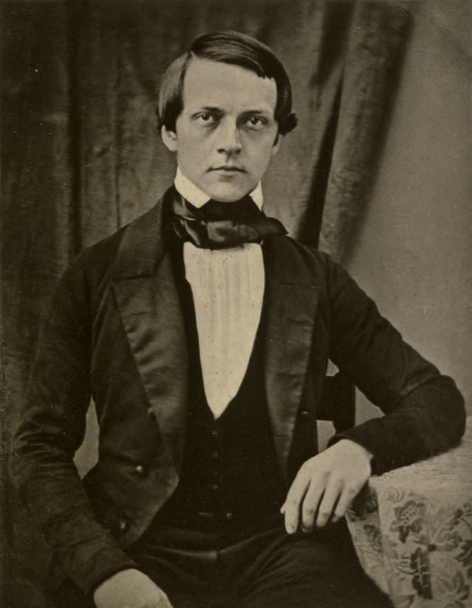
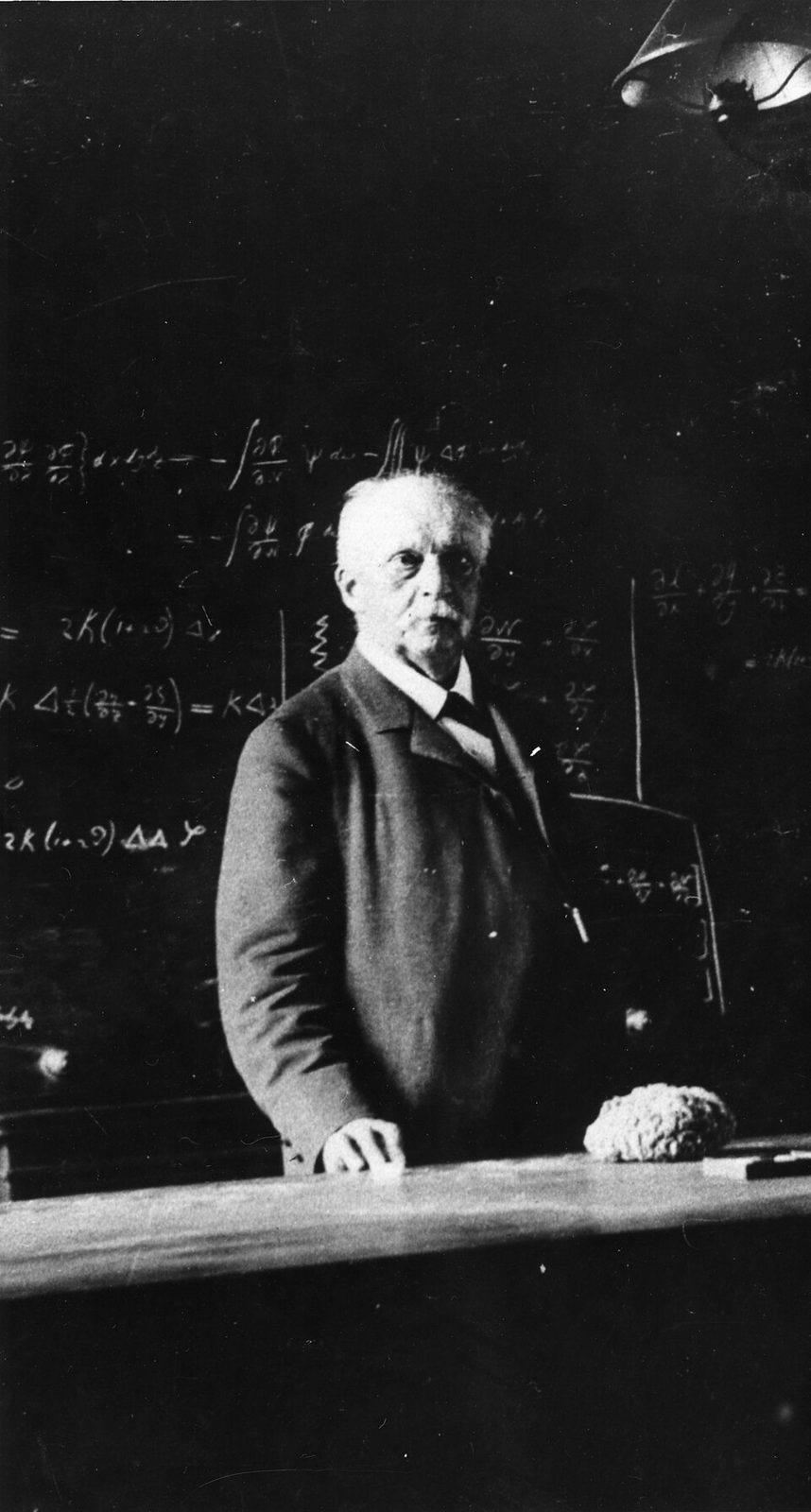
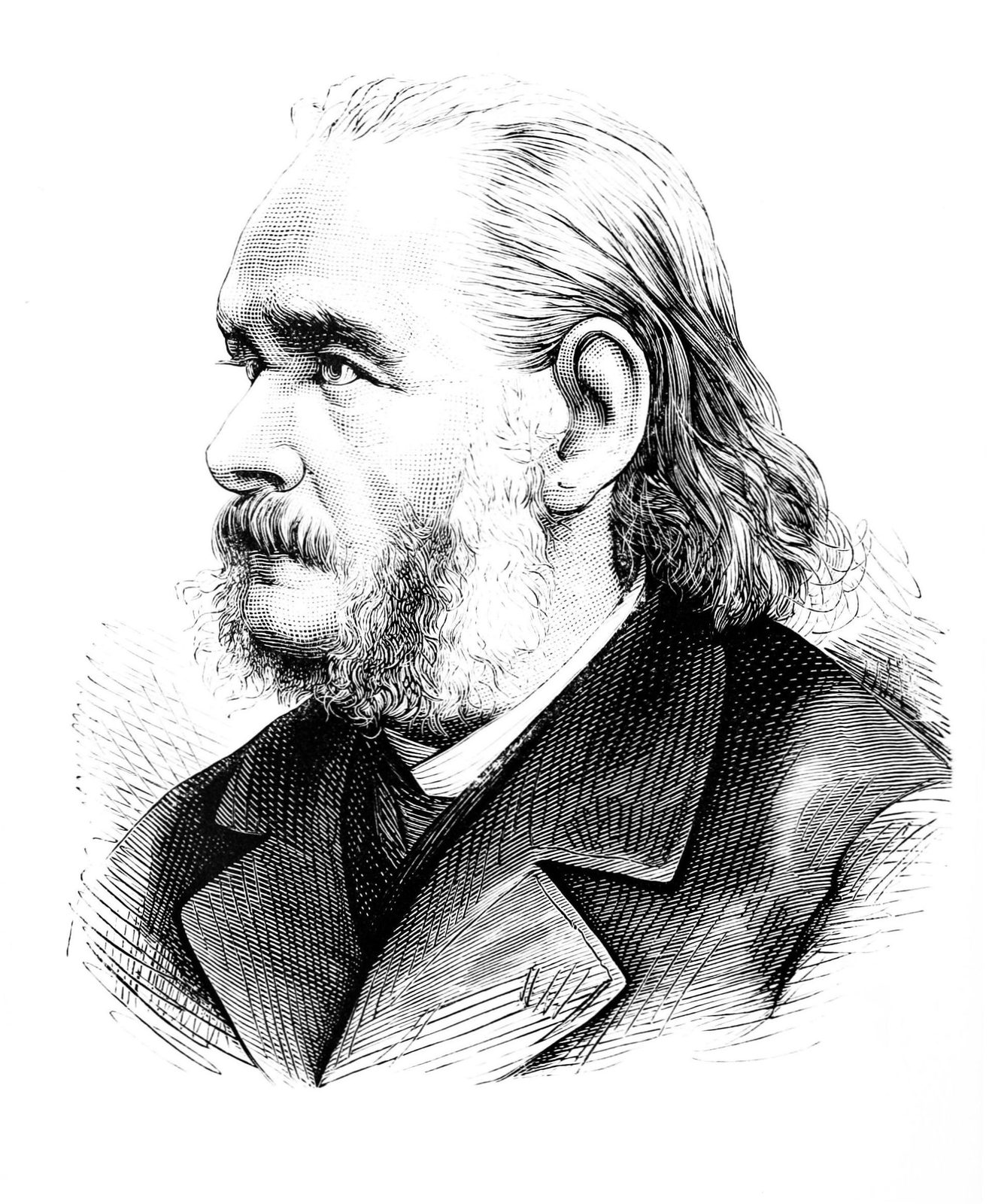
<p class="align-caption"><a href="https://assets.fmusacchio.com/assets/posts/neuroscience/Helmholtz_1848_1600px.jpg" title="Hermann von Helmholtz (1821-1894) in 1848."><img src="https://assets.fmusacchio.com/assets/posts/neuroscience/Helmholtz_1848_800px.jpg" width="58%" alt="Hermann von Helmholtz (1821-1894) in 1848." /></a>
<a href="https://assets.fmusacchio.com/assets/posts/neuroscience/Hermann_von_Helmholtz_photo_1600px.jpg" title="Last photograph of von Helmholtz, taken three days before his final illness."><img src="https://assets.fmusacchio.com/assets/posts/neuroscience/Hermann_von_Helmholtz_photo_800px.jpg" width="40%" alt="Last photograph of von Helmholtz, taken three days before his final illness." /></a><br />
<strong>Left:</strong> Hermann von Helmholtz in 1848. Source: <a href="https://w.wiki/MzEH">Wikimedia Commons</a><span style="color:#d5d6db;font-size:0.8rem;">ꜛ</span> (license: public domain). <strong>Right:</strong> Last photograph of von Helmholtz, taken three days before his final illness. Source: <a href="https://w.wiki/MzEU">Wikimedia Commons</a><span style="color:#d5d6db;font-size:0.8rem;">ꜛ</span> (license: CC0 1.0 Universal Public Domain Dedication). Helmholtz is widely regarded as one of the greatest physicists of the 19th century, and his contributions to physics are foundational. However, his early work on the nervous system is not commonly known and is often overlooked in standard accounts of his scientific career. This is partly because his dissertation was written in Latin and therefore remained largely inaccessible for a long time, but it also reflects a broader tendency in the history of science to reduce scientists to only one part of their intellectual work in my view.</p>

<p>One of the most familiar formulations associated with Helmholtz is the Helmholtz decomposition theorem (in German often just referred to as the Helmholtz theorem). Let’s briefly recall what this is about. In vector calculus, the theorem states that any sufficiently smooth vector field can be decomposed into a divergence-free (solenoidal) part and a curl-free (irrotational) part. Mathematically, for a vector field $\mathbf{F}(\mathbf{x})$ that vanishes at infinity, we can write:</p>

\[\begin{align}
\mathbf{F} &amp;= -\nabla \phi + \nabla \times \mathbf{A}
\end{align}\]

<p>Here, $\phi$ is a scalar potential and $\mathbf{A}$ a vector potential. Physically, this means that any field can be separated into a component that originates from sources or sinks and a component that describes rotational or circulating structures. This decomposition underlies much of classical electrodynamics and <a href="/blog/2021-03-04-hydrodynamics/">fluid dynamics</a>, where electric, magnetic, or velocity fields are naturally described in terms of potentials.</p>

<p>Closely related is the Helmholtz equation, which appears throughout wave physics:</p>

\[\begin{align}
\nabla^2 \psi + k^2 \psi &amp;= 0
\end{align}\]

<p>Here, $\psi$ describes a spatial wave field, such as a sound pressure distribution, an electromagnetic field amplitude, or a quantum mechanical wavefunction. The Laplacian $\nabla^2$ captures how the field changes spatially, while the parameter $k$ is the wave number, related to the wavelength $\lambda$ by</p>

\[\begin{align}
k &amp;= \frac{2\pi}{\lambda}
\end{align}\]

<p>The Helmholtz equation emerges when oscillatory systems are studied in the frequency domain. Instead of describing how a wave evolves in time, it describes the spatial structure of standing or propagating waves at a fixed frequency. Solutions therefore represent spatial wave patterns and resonant modes. The equation appears in acoustics, optics, electrodynamics, and quantum mechanics, but also in <a href="/blog/2020-08-23-space_physics/">plasma physics and space physics</a>, where wave-like disturbances propagate through <a href="/blog/2020-06-05-plasma_characteristics/">magnetized plasmas</a>. <a href="/blog/2020-09-01-plasma_waves/">Plasma waves</a> in the <a href="/blog/2020-08-21-solar_wind_and_parker_spiral/">solar wind</a>, <a href="/blog/2020-09-01-alfven_wave/">magnetospheric oscillations</a>, and electromagnetic wave propagation in ionized media can all lead, under suitable approximations, to Helmholtz-type equations.</p>

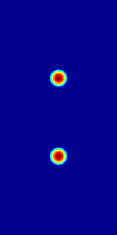
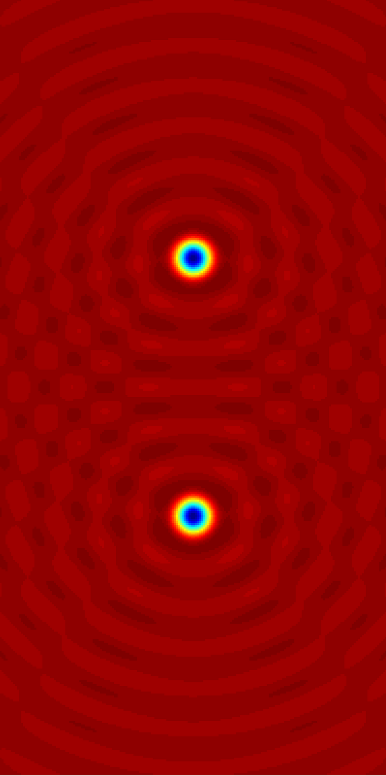
<p class="align-caption"><a href="https://assets.fmusacchio.com/assets/posts/neuroscience/Helmholtz_source_1600px.png" title="Two sources of radiation in the plane."><img src="https://assets.fmusacchio.com/assets/posts/neuroscience/Helmholtz_source_800px.png" width="49.2%" alt="Two sources of radiation in the plane." /></a>
<a href="https://assets.fmusacchio.com/assets/posts/neuroscience/Helmholtz_solution_1600px.png" title="Solution to the inhomogeneous Helmholtz equation."><img src="https://assets.fmusacchio.com/assets/posts/neuroscience/Helmholtz_solution_800px.png" width="49%" alt="Solution to the inhomogeneous Helmholtz equation." /></a><br />
<strong>Left:</strong> Two sources of radiation in the plane, represented mathematically by a source function $f$, which vanishes in the blue region. <strong>Right:</strong> The real part of the resulting field $A$. Here, $A$ is the solution of the inhomogeneous Helmholtz equation $(\nabla^2 + k^2)A = -f$. Source: <a href="https://w.wiki/MzGh">Wikimedia Commons</a><span style="color:#d5d6db;font-size:0.8rem;">ꜛ</span> and <a href="https://w.wiki/MzGm">Wikimedia Commons</a><span style="color:#d5d6db;font-size:0.8rem;">ꜛ</span> (license: public domain). The Helmholtz equation describes how localized sources generate spatial wave fields and interference patterns. Such equations form part of the mathematical foundation of modern wave physics.</p>

<p>Helmholtz’s scientific work, however, extended far beyond vector calculus and wave theory. He also formulated the principle of conservation of energy in a modern quantitative framework, thereby contributing to the unification of mechanics, heat theory, and electromagnetism. At the same time, he remained deeply connected to physiology and medicine throughout his career. In experimental physiology, for example, he famously measured the finite speed of nerve conduction, thereby refuting the older assumption that neural signaling occurred instantaneously. This finding is already remarkable for itself, as at his time, the experiments by <a href="/blog/2024-04-21-hodgkin_huxley_model/">Hodgkin and Huxley</a> that would later provide a detailed mechanistic explanation of nerve conduction were still decades away. But it also illustrates how Helmholtz’s scientific interests spanned both physics and physiology, and how he applied rigorous quantitative methods to the study of biological systems.</p>

<p>So, Helmholtz did not simply move from medicine into physics and leave biology behind. Rather, he approached biological systems with the same quantitative and mechanistic mindset that characterized his physical work. In many ways, he helped establish the broader 19th century idea that physiological processes could be investigated with the tools and methods of physics.</p>

<p>From a physicist’s perspective, Helmholtz is therefore a unifying figure who connects field theory, wave physics, thermodynamics, and physiology. The idea that this same person began his scientific career with a detailed anatomical study of invertebrate nervous systems is therefore unexpected at first glance, but perhaps also strangely fitting.</p>

<h2 id="helmholtzs-dissertation">Helmholtz’s dissertation</h2>
<p>Helmholtz’s 1842 dissertation, <em>De fabrica systematis nervosi evertebratorum</em>, is situated in a specific scientific context. At that time, microscopy had only recently reached a level that allowed the visualization of cellular structures. <a href="https://en.wikipedia.org/wiki/Christian_Gottfried_Ehrenberg">Christian Ehrenberg (1795-1876)</a><span style="color:#d5d6db;font-size:0.8rem;">ꜛ</span> had published the <a href="https://www.researchgate.net/figure/Panel-A-The-structure-of-nerve-tissue-by-Christian-Ehrenberg-1836-Part-a-General_fig5_272076102">first images of neurons</a><span style="color:#d5d6db;font-size:0.8rem;">ꜛ</span> (Ehrenberg (1832, 1836); <a href="https://doi.org/10.1080/0964704X.2014.977676">Chvátal (2015)</a><span style="color:#d5d6db;font-size:0.8rem;">ꜛ</span>), including ganglia of the leech, and the emerging cell theory of <a href="https://en.wikipedia.org/wiki/Matthias_Jakob_Schleiden">Schleiden</a><span style="color:#d5d6db;font-size:0.8rem;">ꜛ</span> and <a href="https://en.wikipedia.org/wiki/Theodor_Schwann">Schwann</a><span style="color:#d5d6db;font-size:0.8rem;">ꜛ</span> proposed that all tissues are composed of cells in 1838/1839 (Schwann (1838); Schwann (1839)).</p>

<p class="align-caption"><a href="https://assets.fmusacchio.com/assets/posts/neuroscience/Ehrenberg_first_imaged_neuron_1600px.png" title="First image of a neuron: A drawing of the leech ganglion by Christian Ehrenberg (1836)."><img src="https://assets.fmusacchio.com/assets/posts/neuroscience/Ehrenberg_first_imaged_neuron_800px.png" width="100%" alt="First image of a neuron: A drawing of the leech ganglion by Christian Ehrenberg (1836)." /></a><br />
First image of a neuron: A drawing of the leech ganglion by Christian Ehrenberg (1836). Individual magnified neurons are displayed on the left. Source: Julia Heideklang, H.-J. Pflüger, Helmut Kettenmann, <a href="https://www.helmholtz.de/fileadmin/user_upload/03_ueber_uns/hermann_von_helmholtz/Helmholtz_Dissertation_wbg_Academic_CC_BY_SA.pdf"><em>De fabrica systematis nervosi evertebratorum. Die kommentierte Dissertation von Hermann Helmholtz</em></a>, 2021, page 10, (license: CC BY-SA 4.0).</p>

<p class="align-caption"><a href="https://assets.fmusacchio.com/assets/posts/neuroscience/Schwann_Theodore_1600px.jpg" title="Theodore Schwann (1810-1882)."><img src="https://assets.fmusacchio.com/assets/posts/neuroscience/Schwann_Theodore_800px.jpg" width="46%" alt="Theodore Schwann (1810-1882)." /></a>
<a href="https://assets.fmusacchio.com/assets/posts/neuroscience/Jacob_Schleiden_1600px.jpg" title="Matthias Schleiden (1804-1881)."><img src="https://assets.fmusacchio.com/assets/posts/neuroscience/Jacob_Schleiden_800px.jpg" width="52.5%" alt="Matthias Schleiden (1804-1881)." /></a><br />
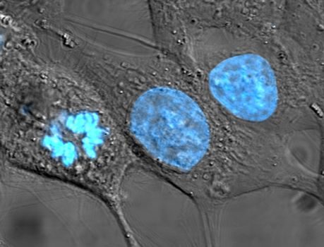
<a href="https://assets.fmusacchio.com/assets/posts/neuroscience/HeLa_cells_stained_with_Hoechst_1600px.jpg" title="HeLa cells stained with Hoechst."><img src="https://assets.fmusacchio.com/assets/posts/neuroscience/HeLa_cells_stained_with_Hoechst_800px.jpg" width="100%" alt="HeLa cells stained with Hoechst." /></a><br />
<strong>Top Left:</strong> Theodore Schwann (1810-1882); from <em>The Story of Nineteenth-Century Science</em>, page 377, 1904, by Henry Smith Williams. Source: <a href="https://w.wiki/MzCL">Wikimedia Commons</a><span style="color:#d5d6db;font-size:0.8rem;">ꜛ</span> (license: public domain). <strong>Top Right:</strong> Matthias Schleiden (1804-1881), between 1882 and 1883. Source: <a href="https://w.wiki/MzCT">Wikimedia Commons</a><span style="color:#d5d6db;font-size:0.8rem;">ꜛ</span> (license: public domain). <strong>Bottom:</strong> Human cancer cells with nuclei (specifically the DNA) stained blue. The central and rightmost cell are in interphase, so the entire nuclei are labeled. The cell on the left is going through mitosis and its DNA has condensed. Source: <a href="https://w.wiki/MzC$">Wikimedia Commons</a><span style="color:#d5d6db;font-size:0.8rem;">ꜛ</span> (license: public domain). – Schwann and Schleiden are credited with the formulation of the cell theory, which posits that all living organisms are composed of cells. This was a foundational concept in biology, and it set the stage for later investigations into the cellular structure of tissues, including the nervous system. Helmholtz’s dissertation can be seen as an early attempt to apply these emerging ideas to the study of nervous tissue in invertebrates.</p>

<p>However, while vertebrate nervous systems had begun to be described, a systematic investigation of invertebrate nervous systems was largely missing. Helmholtz’s supervisor, <a href="https://en.wikipedia.org/wiki/Johannes_Peter_Müller">Johannes Müller</a><span style="color:#d5d6db;font-size:0.8rem;">ꜛ</span>, assigned precisely this problem to the young medical student: To determine whether the structural principles of nervous systems are conserved across species.</p>

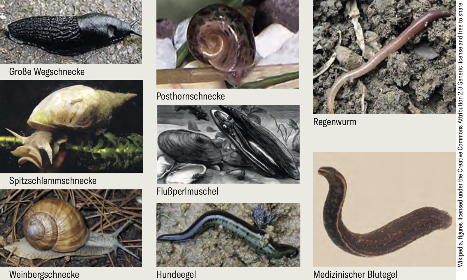
<p class="align-caption"><a href="https://assets.fmusacchio.com/assets/posts/neuroscience/Helmholtz_Experimental_animals_1600px.png" title="Nervous system of the Medicinal leech."><img src="https://assets.fmusacchio.com/assets/posts/neuroscience/Helmholtz_Experimental_animals_800px.png" width="100%" alt="Nervous system of the Medicinal leech." /></a><br />
Experimental animals used by Helmholtz in his dissertation: Giant slug (<em>Arion empiricorum</em>; today: <em>Arion ater</em>), Great pond snail (<em>Limnaea stagnalis</em>), Burgundy snail (<em>Helix pomatia</em>), Great ramshorn snail (<em>Planorbis corneus</em>; today: <em>Planorbarius corneus</em>), Freshwater pearl mussel (<em>Unio margaritifera</em>; today: <em>Margaritifera margaritifera</em>), Common leech (<em>Hirudo vulgaris</em>), Earthworm (<em>Lumbricus terrestris</em>), Medicinal leech (<em>Hirudo medicinalis</em>). Source: Julia Heideklang, H.-J. Pflüger, Helmut Kettenmann, <a href="https://www.helmholtz.de/fileadmin/user_upload/03_ueber_uns/hermann_von_helmholtz/Helmholtz_Dissertation_wbg_Academic_CC_BY_SA.pdf"><em>De fabrica systematis nervosi evertebratorum. Die kommentierte Dissertation von Hermann Helmholtz</em></a>, 2021, page 14, (license: CC BY-SA 4.0).</p>

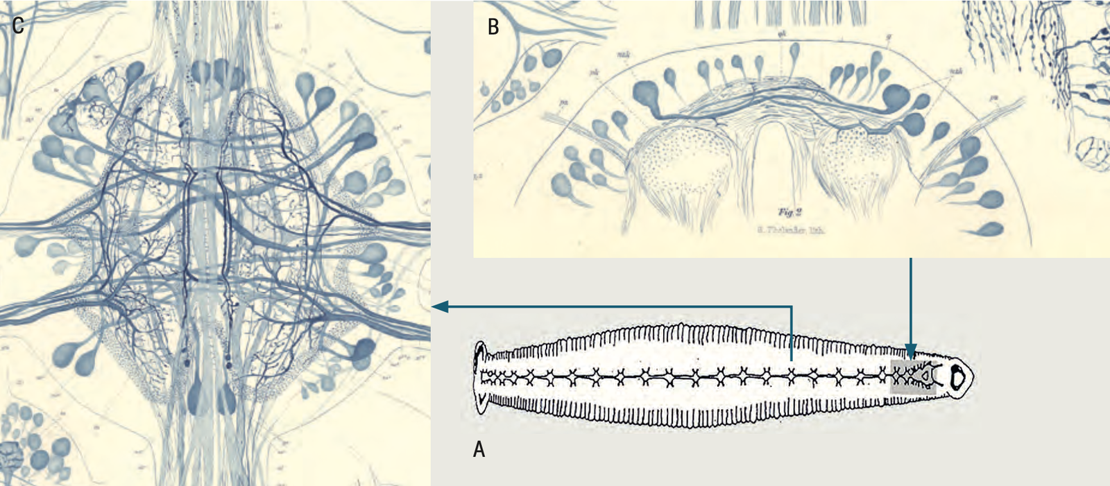
<p>Helmholtz approached this question through comparative anatomical analysis of a range of invertebrates, including leeches, worms, crustaceans, and insects. His method was fundamentally microscopic dissection and observation. For example, he describes how a nerve or nerve cord, taken from a living animal and mechanically separated on a glass plate, reveals individual nerve fibers under appropriate preparation. Similarly, by dissecting ganglia, he identifies cellular structures, including what he describes as “caudate cells”, that is, cell bodies with extensions.</p>

<p class="align-caption"><a href="https://assets.fmusacchio.com/assets/posts/neuroscience/Helmholtz_Nervous_system_of_the_Medicinal_leech_1600px.png" title="Nervous system of the Medicinal leech."><img src="https://assets.fmusacchio.com/assets/posts/neuroscience/Helmholtz_Nervous_system_of_the_Medicinal_leech_800px.png" width="100%" alt="Nervous system of the Medicinal leech." /></a><br />
Nervous system of the Medicinal leech. (A) Scheme of the nervous system; (B) Upper part of the supraesophageal
ganglion (brain); (C) Fourth ganglion of the ventral nerve cord; Retzius 1891. Helmholtz describes the nervous system of the leech in detail, identifying nerve cords, ganglia, and cellular structures. This figure from Retzius (1891) illustrates the organization of the leech nervous system, which Helmholtz would have studied in his dissertation. Source: Julia Heideklang, H.-J. Pflüger, Helmut Kettenmann, <a href="https://www.helmholtz.de/fileadmin/user_upload/03_ueber_uns/hermann_von_helmholtz/Helmholtz_Dissertation_wbg_Academic_CC_BY_SA.pdf"><em>De fabrica systematis nervosi evertebratorum. Die kommentierte Dissertation von Hermann Helmholtz</em></a>, 2021, page 19, (license: CC BY-SA 4.0).</p>

<p>Thus, Helmholtz is effectively describing neurons as entities consisting of a cell body and processes, without yet having the conceptual framework of the neuron doctrine (the principle that the nervous system consists of distinct individual neurons rather than a continuous network). The terminology is not modern, but the observational content clearly anticipates it.</p>

<p>A central structural motif in his analysis is the organization of nerve cords and ganglia. He identifies longitudinal nerve cords connected by ganglia and observes that these ganglia contain lobed structures receiving nerve fibers from the cords. He further describes plexus-like arrangements, where multiple nerve branches interconnect and exchange fibers, in a manner analogous to plexuses in vertebrates.</p>

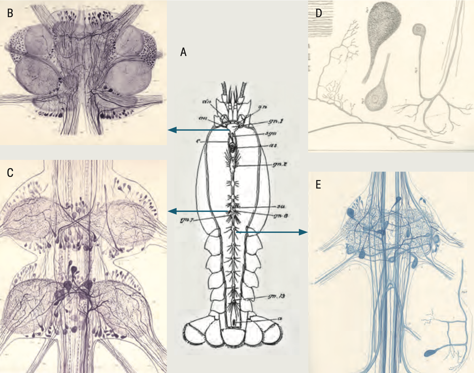
<p>One of the most significant conceptual conclusions of the dissertation is the assertion of structural homology between invertebrate and vertebrate nervous systems. Helmholtz argues that, despite differences in overall organization, the fundamental elements are the same. Nerve fibers, cellular bodies, and their interconnections follow a common structural plan across species. This is explicitly reflected in his comparison of branching patterns in invertebrate nerve plexuses to those found in vertebrates, where each branch carries fibers corresponding to those entering and leaving connected structures.</p>

<p class="align-caption"><a href="https://assets.fmusacchio.com/assets/posts/neuroscience/Huxley_1880_1600px.png" title="Nervous system of the crayfish."><img src="https://assets.fmusacchio.com/assets/posts/neuroscience/Huxley_1880_800px.png" width="100%" alt="Nervous system of the crayfish." /></a><br />
Nervous system of the crayfish after Huxley (1880): (A) Scheme of the nervous system (Retzius 1890), (B) Supraesophageal ganglion (brain), (Retzius 1890), (C) Third thoracic ganglion (Retzius 1890), (D) Individual nerve cells (Retzius 1890), (E) First abdominal ganglion (Retzius 1890). Helmholtz argues in his dissertation that the structural organization of the nervous system in invertebrates, such as the crayfish, shares fundamental features with vertebrate nervous systems: Nerve fibers, ganglia, and plexus-like arrangements are common motifs that reflect a shared structural plan. Source: Julia Heideklang, H.-J. Pflüger, Helmut Kettenmann, <a href="https://www.helmholtz.de/fileadmin/user_upload/03_ueber_uns/hermann_von_helmholtz/Helmholtz_Dissertation_wbg_Academic_CC_BY_SA.pdf"><em>De fabrica systematis nervosi evertebratorum. Die kommentierte Dissertation von Hermann Helmholtz</em></a>, 2021, page 21, (license: CC BY-SA 4.0).</p>

<p>In modern terms, this can be interpreted as an early formulation of a unifying principle of nervous system organization: That neural circuits are constructed from recurring cellular and connective motifs, independent of the organism. This is not yet an evolutionary argument in the Darwinian sense, but it is clearly a structural generalization across species.</p>

<p>Another important aspect is actually methodological. Helmholtz relies on careful mechanical dissection, microscopy, and comparative reasoning. There is no <a href="/blog/2022-10-13-Read_ibw_files/">electrophysiology</a>, no staining techniques in the modern sense, and no formal theory of <a href="/blog/2026-02-12-stdp/">synaptic connectivity</a>. Yet, within these constraints, he identifies consistent structural patterns and interprets them in a general framework.</p>

<p>It is also crucial to emphasize what is absent. As mentioned in the introduction, there is no distinction between neurons and glial cells, because this conceptual separation had not yet been introduced. The nervous system is treated as a collection of fibers and cellular elements without a clear functional differentiation between support and signaling components. This absence highlights how early Helmholtz’s work is situated within the development of neuroscience.</p>

<p>What also surprised me is the absence of any figures in the dissertation. The text in this new translation is entirely descriptive, both in the original Latin version and in the translation, and while it contains detailed descriptions of structures, there are no illustrations or diagrams. This is quite different from what we know from today’s scientific publications, where figures play a central role in conveying information. At the moment, I can’t rule out whether this was an editorial choice in the translation or whether the original dissertation also lacked figures. But either way, it emphasizes the textual and descriptive nature of scientific communication at that time. If you have already seen other scientific texts from the early 19th century, you might know that this was not uncommon. The detailed descriptions of concepts and observations were conveyed entirely through words, which is a significant difference from modern scientific writing.</p>

<p>Taken together, the dissertation can be understood as an early comparative neuroanatomical study that establishes three key points:</p>

<ol>
  <li>First, nervous systems across different animal classes share a common structural basis.</li>
  <li>Second, these systems are composed of cellular elements and fibers that can be identified microscopically.</li>
  <li>Third, their organization into ganglia, cords, and plexuses follows systematic and reproducible patterns.</li>
</ol>

<p>These insights, while not yet framed in the language of modern neuroscience, clearly anticipate later developments in the understanding of nervous system structure and organization. Helmholtz’s work can therefore be seen as a foundational contribution to the field, even if it has been largely overlooked in standard historical accounts.</p>

<h2 id="conclusion">Conclusion</h2>
<p>What remains, after reading this dissertation in light of Helmholtz’s later work, is a certain sense of discontinuity that is, in fact, highly revealing. The figure who would later formalize energy conservation, develop mathematical frameworks for fields and waves, and shape theoretical physics, begins with meticulous anatomical observations of leeches and worms under a microscope.</p>

<p>From a modern perspective, this is not merely an anecdotal curiosity. It reflects a broader feature of 19th century science (and even in earlier times), where disciplinary boundaries were not yet rigidly established. The same individual could move from cell structure to electrodynamics without the conceptual friction that would exist today. Other famous figures such as Carl Friedrich Gauss, Michael Faraday, and James Clerk Maxwell also had similarly broad scientific interests that spanned multiple fields.</p>

<p>At the same time, the dissertation itself is more than a historical footnote. It contains a clear recognition of structural unity across nervous systems and an implicit cellular perspective that anticipates later developments. That this work was written in Latin and remained largely inaccessible for nearly two centuries may explain why it has not entered the standard narrative of neuroscience.</p>

<p>And Kettenmann’s remark on this work, in retrospect, points to something more general: The early history of neuroscience was less linear than our retrospective narratives often suggest. Ideas that now seem closely connected, such as cell theory, comparative neuroanatomy, glia, neurons, and physiological mechanism, did not emerge as one coherent program. They developed in fragments, in different disciplines, with different terminologies and different methods. Helmholtz’s early contribution to neuroscience was neither trivial nor naive. It was one such fragment. Revisiting it does not change the established milestones of neuroscience, but it does refine the picture. It shows that some of the core ideas about the cellular organization and comparative structure of nervous systems were already being articulated at a time when even the basic terminology had not yet been established.</p>

<p>Personally, this is also why I find Helmholtz’s scientific trajectory so interesting. I began in physics myself and later moved into neuroscience, although, of course, in a completely different historical and scientific context. For that reason, the trajectory from physical thinking to biological questions feels familiar, and reminds me that the border between physics and neuroscience is not as sharp as it sometimes appears. Helmholtz’s dissertation makes this visible in an unusually early and concrete form: The nervous system was already a place where anatomy, physiology, microscopy, and physical reasoning could meet.</p>

<p>As mentioned at the beginning, the new translation is <a href="https://www.helmholtz.de/ueber-uns/wer-wir-sind/geschichte/helmholtz-dissertation/">shared</a><span style="color:#d5d6db;font-size:0.8rem;">ꜛ</span> under a Creative Commons license and is <a href="https://www.helmholtz.de/fileadmin/user_upload/03_ueber_uns/hermann_von_helmholtz/Helmholtz_Dissertation_wbg_Academic_CC_BY_SA.pdf">freely available online</a><span style="color:#d5d6db;font-size:0.8rem;">ꜛ</span>. For anyone interested in the history of neuroscience, physiology, or 19th century science more broadly, it is well worth reading. Feel free to share your thoughts and insights in the <a href="#comments">comments below</a>.</p>

<h2 id="references-and-further-reading">References and further reading</h2>
<ul>
  <li>Julia Heideklang, H.-J. Pflüger, Helmut Kettenmann, <em>De fabrica systematis nervosi evertebratorum. Die kommentierte Dissertation von Hermann Helmholtz</em>, 2021, Wbg Academic, ISBN: 9783534400942, <a href="https://www.helmholtz.de/fileadmin/user_upload/03_ueber_uns/hermann_von_helmholtz/Helmholtz_Dissertation_wbg_Academic_CC_BY_SA.pdf">online PDF</a><span style="color:#d5d6db;font-size:0.8rem;">ꜛ</span>, <a href="https://www.helmholtz.de/ueber-uns/wer-wir-sind/geschichte/helmholtz-dissertation/">Website</a><span style="color:#d5d6db;font-size:0.8rem;">ꜛ</span></li>
  <li>Chvátal, A., <em>Discovering the Structure of Nerve Tissue: Part 1: From Marcello Malpighi to Christian Berres</em>, 2015, Journal of the History of the Neurosciences, 24(3), 268–291. doi: <a href="https://doi.org/10.1080/0964704X.2014.977676">10.1080/0964704X.2014.977676</a><span style="color:#d5d6db;font-size:0.8rem;">ꜛ</span></li>
  <li>Ehrenberg, C. G., <em>Über das neueste Mikroskop, von Pistor und Schiek in Berlin, gefertigt im Januar 1832</em>, 1832, Ein Schreiben von Hrn. Ehrenberg an den Herausgeber, Januarheft 1832 der Analen der Physik, 188-192</li>
  <li>Ehrenberg, C. G., <em>Abhandlung der Akademie: Beobachtung einer bisher unbekannren auffallenden Structur des Seelenorgans bei Menschen und Thieren</em>, 1836, Berlin</li>
  <li>Schleiden, M., <em>Beträge zur Phytogenesis</em>, 1838, Archiv für Anatomie, Physiologie und wissenschaftliche Medicin, Weit et Comp. Berlin</li>
  <li>Schwann, T., <em>Mikroskopische Untersuchungen über die Übereinstimmung in der Struktur und dem Wachstum der Thiere und Pflanzen</em>, 1839, Sander’sche Buchhandlung, Berlin</li>
  <li>Rudolf Virchow, <em>Die Cellularpathologie in ihrer Begründung auf physiologische und pathologische Gewebelehre: Zwanzig Vorlesungen, gehalten während der Monate Februar, März und April 1858 im pathologischen Institute zu Berlin</em>, 1856, Verlag von August Hirschwald, Berlin</li>
</ul>

<!-- 
Write a Mastodon post summarizing this article in an objective, academic tone. Don't write ABOUT the article, but about its content/topic. (max. 450 characters + URL, which follows this scheme: https://www.fabriziomusacchio.com/blog/[FILE-NAME_WITHOUT_FILE-EXTENSION]/):

To my surprise, I recently learned that Hermann von #Helmholtz’s 1842 dissertation was not about #physics, but about the #NervousSystem. It was an anatomical study of invertebrate nervous systems, written at a time when the conceptual distinction between #neurons and #glia did not yet exist.

I wrote a short blog post about this fascinating early contribution to #neuroscience:

🌍 https://www.fabriziomusacchio.com/blog/2026-05-09-helmholtz_dissertation/

#Neuroscience #ScienceHistory

--- 

Reading the dissertation was fascinating because it reveals a side of #Helmholtz that is rarely discussed today. Long before his work on #EnergyConservation, #electrodynamics, and #WavePhysics, he was already deeply engaged with #anatomical and #biological questions.

It also shows that some core ideas about the comparative structure of nervous systems were already being articulated in the early 19th century.

#Neuroscience #Physics #ScienceHistory

--- 

Always striking to see how multi-faceted some of the great scientists of the past were (#Gauss, #Faraday, #Maxwell, #Newton, #Somerville, #Lovelace etc.). The boundaries between disciplines were much more fluid back then, and the same person could contribute to multiple fields, even though they might be remembered for only one today.

#Neuroscience #Physics #ComputerScience #Mathematics #Biology #Astronomy #Geophysics #ScienceHistory

--- 

And btw, Helmholtz’s translated dissertation is freely available online under a Creative Commons license, thanks to Julia Heideklang, H.-J. Pflüger, and Helmut Kettenmann, who made this early work accessible again by translating it from Latin into English and German:

🌍 https://www.helmholtz.de/ueber-uns/wer-wir-sind/geschichte/helmholtz-dissertation/
📕 https://www.helmholtz.de/fileadmin/user_upload/03_ueber_uns/hermann_von_helmholtz/Helmholtz_Dissertation_wbg_Academic_CC_BY_SA.pdf

-->]]></content><author><name> </name></author><category term="Physics" /><category term="Neuroscience" /><category term="Personal Opinion" /><summary type="html"><![CDATA[While Hermann von Helmholtz is widely known for his foundational contributions to physics, his early scientific work was actually focused on the nervous system. In this post, I share insights from reading Helmholtz's 1842 dissertation, which was recently translated from Latin into English by Helmut Kettenmann and colleagues. The dissertation reveals Helmholtz's detailed anatomical study of invertebrate nervous systems, conducted at a time when the conceptual distinction between neurons and glial cells did not yet exist.]]></summary></entry><entry><title type="html">Clopath plasticity rule</title><link href="/blog/2026-04-14-clopath_rule/" rel="alternate" type="text/html" title="Clopath plasticity rule" /><published>2026-04-14T09:44:41+02:00</published><updated>2026-04-14T09:44:41+02:00</updated><id>/blog/clopath_rule</id><content type="html" xml:base="/blog/2026-04-14-clopath_rule/"><![CDATA[<p>The Clopath learning rule is a biophysically inspired model of <a href="/blog/2026-02-02-neural_plasticity_and_learning/">synaptic plasticity</a> that extends classical <a href="/blog/2024-03-03-hebbian_learning_and_hopfield_networks/">Hebbian learning</a> and simple <a href="/blog/2026-02-12-stdp/">spike-timing-dependent plasticity (STDP)</a> formulations by incorporating the postsynaptic membrane voltage as an explicit state variable. Introduced by <a href="https://doi.org/10.1038/nn.2479">Claudia Clopath et al. in 2010</a><span style="color:#d5d6db;font-size:0.8rem;">ꜛ</span>, the rule was designed to account for experimental findings that cannot be captured well by timing-only STDP rules. In particular, synaptic potentiation and depression do not depend only on the relative timing of pre- and postsynaptic spikes, but also on the depolarization state of the postsynaptic neuron.</p>

<p class="align-caption"><img src="https://assets.fmusacchio.com/assets/posts/neural_dynamics/clopath_synapse_spike_pairing_1600px.png" alt="jpg" title="Clopath plasticity rule" class="align-center_80" />
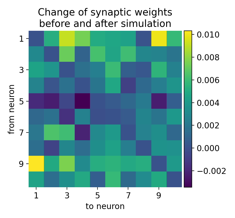
Result of a spike pairing simulation using the Clopath rule. The plot shows the change in synaptic weight as a function of the relative timing of pre- and postsynaptic spikes. The Clopath rule captures both potentiation and depression of synaptic weights based on the timing of spikes and the postsynaptic membrane potential. We will simulate this experiment in the section “Spike pairing simulation” below.</p>
<p>This makes the Clopath rule especially important in <a href="/blog/2026-02-04-neural_dynamics/">computational neuroscience</a>. It provides a compact phenomenological framework that links <a href="/blog/2026-02-02-neural_plasticity_and_learning/">synaptic plasticity</a> to membrane dynamics, spike timing, and homeostatic stabilization. As a result, it is widely used in spiking neural network simulations that aim to remain closer to biological plasticity mechanisms than pair-based <a href="/blog/2026-02-12-stdp/">STDP rules</a>.</p>

<h2 id="mathematical-description">Mathematical description</h2>
<p>The central idea of the Clopath rule is that <a href="/blog/2024-09-15-ltp_and_ltd/">potentiation and depression</a> depend on different combinations of presynaptic activity and postsynaptic voltage. In contrast to simple <a href="/blog/2026-02-12-stdp/">STDP rules</a>, the postsynaptic membrane potential is not treated as an implicit byproduct of spike times, but as a relevant dynamical quantity in its own right.</p>

<p>A simplified schematic form of the rule can be written as</p>

\[\begin{align*}
\frac{dw_{ij}}{dt} =&amp; -A_\text{LTD} \, x_i(t)\,[\bar{u}_j(t)-\theta_-]_+ \\
&amp; + A_\text{LTP} \, \bar{x}_i(t)\,[u_j(t)-\theta_+]_+[\bar{u}_j(t)-\theta_-]_+,
\end{align*}\]

<p>where</p>

<ul>
  <li>$w_{ij}$ is the synaptic weight from presynaptic neuron $i$ to postsynaptic neuron $j$,</li>
  <li>$A_\text{LTD}$ and $A_\text{LTP}$ set the relative strength of the depressive and potentiating plasticity components,</li>
  <li>$x_i(t)$ and $\bar{x}_i(t)$ are presynaptic traces,</li>
  <li>$u_j(t)$ is the postsynaptic membrane potential,</li>
  <li>$\bar{u}_j(t)$ is a low pass filtered postsynaptic voltage,</li>
  <li>$\theta_-$ and $\theta_+$ are voltage thresholds for depression and potentiation, respectively, and</li>
  <li>$[\,\cdot\,]_+ = \max(\cdot,0)$ denotes rectification.</li>
</ul>

<p>This expression captures the main logic of the model:</p>

<ul>
  <li>depression is triggered when presynaptic activity coincides with sufficient postsynaptic depolarization above a lower threshold</li>
  <li>potentiation requires stronger postsynaptic depolarization above a higher threshold and depends on presynaptic activation through a trace term</li>
  <li>the two processes are therefore asymmetric in their voltage dependence</li>
</ul>

<p>The precise formulation differs somewhat between the original papers and specific simulator implementations such as NEST (see below), but the conceptual structure remains the same.</p>

<p>A typical presynaptic trace is described by</p>

\[\frac{dx_i(t)}{dt} = -\frac{x_i(t)}{\tau_x} + \sum_f \delta(t-t_i^f),\]

<p>where $\tau_x$ is the decay time constant and $t_i^f$ denotes the times of presynaptic spikes. $\delta(t - t_i^f)$ represents the Dirac delta function indicating a presynaptic spike at time $t_i^f$. $f$ denotes the time of the presynaptic spike. The (low-pass) filtered <a href="/blog/2026-02-12-stdp/#synapse">postsynaptic</a> voltage potential can be written as</p>

\[\frac{d\bar{u}_j(t)}{dt} = -\frac{\bar{u}_j(t)}{\tau_u} + u_j(t),\]

<p>where $\tau_u$ is the corresponding voltage filter (decay) time constant.</p>

<p>In addition to its voltage dependence, the original Clopath model also contains a homeostatic component that prevents runaway synaptic growth. This is one of the key reasons why the rule is more stable in recurrent network simulations than many simpler <a href="/blog/2026-02-12-stdp/">STDP variants</a>.</p>

<p>The synaptic weights are typically bounded such that</p>

\[0 \leq w_{ij} \leq w_\text{max}.\]

<p>In some versions of the model, the <a href="/blog/2024-09-15-ltp_and_ltd/">LTD</a> amplitude is further modulated by a homeostatic postsynaptic activity term, for example in the schematic form</p>

\[A_\text{LTD} \propto \alpha \frac{\bar{u}_{j,\mathrm{homeo}}^2}{u_\text{ref}^2},\]

<p>where $\alpha$ is a scaling factor, $u_\text{ref}$ is a reference level, and $\bar{u}_{j,\mathrm{homeo}}$ denotes a slowly varying postsynaptic activity or voltage measure rather than the instantaneous membrane potential itself. The exact form depends on the specific model variant or simulator implementation.  This allows the rule to counteract runaway potentiation and helps maintain stable learning in recurrent networks.</p>

<h2 id="implementation-in-neural-network-simulations">Implementation in neural network simulations</h2>
<p>To use the Clopath rule in a spiking network simulation, one must supply not only <a href="/blog/2026-02-12-stdp/#synapse">pre- and postsynaptic spikes</a> but also the postsynaptic membrane voltage and its filtered versions. For this reason, the rule is often coupled to a neuron model that provides a realistic subthreshold voltage trajectory. A common choice is the <a href="/blog/2024-08-25-EIF_and_AdEx_model/#derivation-of-the-adex-model">adaptive exponential integrate and fire (AdEx) neuron model</a>, which captures leak dynamics, exponential spike initiation, and adaptation. A standard AdEx membrane equation is</p>

\[\begin{align*}
C \frac{du(t)}{dt} = &amp; -g_L \bigl(u(t)-E_L\bigr) + g_L \Delta_T e^{(u(t)-V_T)/\Delta_T} \\
 &amp; - I_\text{adapt}(t) + I_\text{syn}(t) + I_\text{ext}(t),
\end{align*}\]

<p>where $u(t)$ is the membrane potential, $C$ is the membrane capacitance, $g_L$ is the leak conductance, $E_L$ is the resting potential, $\Delta_T$ controls the sharpness of spike initiation, $V_T$ is the (adaptive) threshold parameter, $I_\text{adapt}(t)$ is the adaptation current, $I_\text{syn}(t)$ is the synaptic current, and $I_\text{ext}(t)$ is the external input current.</p>

<p>The adaptation current is commonly modeled as</p>

\[\frac{dI_\text{adapt}(t)}{dt} = \frac{a\bigl(u(t)-E_L\bigr)-I_\text{adapt}(t)}{\tau_\text{adapt}},\]

<p>where $a$ is the adaptation conductance and $\tau_\text{adapt}$ is the adaptation time constant.</p>

<p>In the context of the Clopath rule, the <a href="/blog/2026-02-12-stdp/#synapse">synaptic</a> current $I_\text{syn}(t)$ is given by the sum of inputs from all presynaptic neurons, weighted by their synaptic weights $w_{ij}$:</p>

\[I_\text{syn}(t) = \sum_i w_{ij} \cdot x_i(t).\]

<p>In this setting, the Clopath synapse does not replace the neuron model. Rather, it uses the neuron model’s voltage trajectory to determine when <a href="/blog/2024-09-15-ltp_and_ltd/">synaptic potentiation or depression</a> should occur. This separation is important conceptually: The <a href="/blog/2024-08-25-EIF_and_AdEx_model/">AdEx model</a> describes membrane dynamics, whereas the Clopath rule describes <a href="/blog/2026-02-02-neural_plasticity_and_learning/">plasticity at synapses</a>.</p>

<p>In some <a href="/blog/2024-08-25-EIF_and_AdEx_model/">AdEx</a>-based implementations, the threshold potential is itself adaptive and evolves dynamically after each spike. A simple phenomenological form is</p>

\[\frac{dV_T(t)}{dt} = -\frac{V_T(t)-V_{T,\infty}}{\tau_{V_T}},\]

<p>where $V_{T,\infty}$ is the baseline threshold value and $\tau_{V_T}$ is the corresponding relaxation time constant.</p>

<p>In <a href="https://doi.org/10.3389/fnsyn.2010.00025">Clopath and Gerstner (2010)</a><span style="color:#d5d6db;font-size:0.8rem;">ꜛ</span>, the interaction between spike timing and voltage was further analyzed in a formulation that includes a depolarizing spike afterpotential. This can be represented by an additional variable $z(t)$ that is incremented at spike times and otherwise decays exponentially:</p>

\[\frac{dz(t)}{dt} = -\frac{z(t)}{\tau_z}.\]

<p>Such additions are useful because they help reproduce experimental pairing protocols more faithfully.</p>

<h2 id="why-the-clopath-rule-matters">Why the Clopath rule matters</h2>
<p>The Clopath learning rule is significant for several reasons:</p>

<h3 id="biological-plausibility">Biological plausibility</h3>
<p>A major advantage of the Clopath rule is that it links synaptic modification to the postsynaptic voltage state. This reflects the fact that in biological neurons, <a href="/blog/2026-02-02-neural_plasticity_and_learning/">synaptic plasticity</a> is shaped not only by spike timing but also by dendritic and somatic depolarization. In this sense, the rule is substantially closer to experimentally observed plasticity than purely timing-based <a href="/blog/2026-02-12-stdp/">STDP models</a>.</p>

<h3 id="voltage-dependence">Voltage dependence</h3>
<p>The model distinguishes between weaker depolarization regimes associated with <a href="/blog/2024-09-15-ltp_and_ltd/">depression</a> and stronger depolarization regimes associated with <a href="/blog/2024-09-15-ltp_and_ltd/">potentiation</a>. This captures an important principle of real <a href="/blog/2026-02-12-stdp/#synapse">synapses</a>: The effect of presynaptic input depends on the electrical state of the postsynaptic cell. The same presynaptic spike train can therefore induce very different weight changes depending on whether the postsynaptic neuron is weakly depolarized, strongly depolarized, or near firing threshold.</p>

<h3 id="homeostasis">Homeostasis</h3>
<p>The Clopath model includes homeostatic ingredients that help constrain weight growth and maintain stable activity over time. This is especially important in recurrent networks (RNN), where unconstrained <a href="/blog/2024-03-03-hebbian_learning_and_hopfield_networks/">Hebbian plasticity</a> can otherwise produce runaway excitation or pathological synchrony.</p>

<!-- ### Bidirectional connections
The Clopath rule can establish bidirectional connections because it allows [synaptic weights](/blog/2026-02-12-stdp/#synapse) to be modified in both directions (potentiation and depression) based on the correlation of activities between pre- and postsynaptic neurons. This means that both increasing and decreasing synaptic strengths are possible (bidirectional [plasticity](/blog/2026-02-02-neural_plasticity_and_learning/)), depending on the specific activity patterns. Bidirectional connections have several advantages in neural networks:

* **Network stability and flexibility**: Bidirectional [synaptic plasticity](/blog/2026-02-02-neural_plasticity_and_learning/) allows the network to adapt to changing input patterns while maintaining overall stability. This adaptability is crucial for [learning and memory formation](/blog/2026-02-02-neural_plasticity_and_learning/), as it enables the network to fine-tune connections based on experience.
* **Memory encoding**: The ability to strengthen and weaken synaptic connections bidirectionally is essential for encoding both positive and negative associations. It allows the network to dynamically adjust and store information efficiently.
* **Hebbian learning**: Bidirectional [plasticity](/blog/2026-02-02-neural_plasticity_and_learning/) supports [Hebbian learning principles](/blog/2024-03-03-hebbian_learning_and_hopfield_networks/) ("cells that fire together, wire together" and "cells out of sync, lose their link"). The Clopath rule provides a biologically plausible mechanism for implementing these principles, ensuring that [synaptic changes](/blog/2026-02-12-stdp/#synapse) are activity-dependent and temporally precise. -->

<h3 id="computational-usefulness">Computational usefulness</h3>
<p>From a <a href="/blog/2026-02-04-neural_dynamics/">modeling</a> perspective, the Clopath rule is attractive because it remains relatively compact while capturing several important experimental dependencies. In particular, it provides a practical compromise between biological realism and computational tractability: It goes beyond purely timing-based <a href="/blog/2026-02-12-stdp/">STDP</a> rules by incorporating postsynaptic voltage, yet remains simple enough to be used in larger spiking network simulations. This makes it useful in studies of receptive field formation, self-organization, synaptic competition, and activity-dependent structure in recurrent circuits. Because each synapse is updated locally on the basis of presynaptic activity and the postsynaptic voltage state, even reciprocal connections between two neurons do not have to evolve symmetrically. In this way, the rule can contribute to the emergence of structured and direction-specific connectivity patterns rather than merely uniform global weight changes. Whenever a plasticity model is needed that depends on more than spike timing alone, the Clopath rule is a natural candidate.</p>

<h2 id="spike-pairing-simulation">Spike pairing simulation</h2>
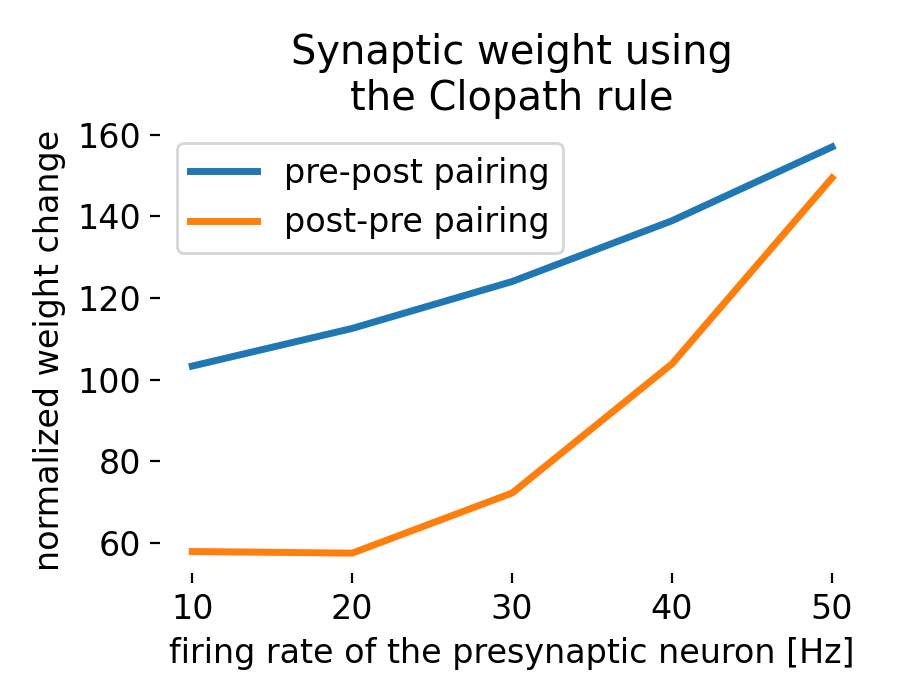
<p>The Clopath rule (<a href="https://nest-simulator.readthedocs.io/en/stable/models/clopath_synapse.html"><code class="language-plaintext highlighter-rouge">clopath_synapse</code></a><span style="color:#d5d6db;font-size:0.8rem;">ꜛ</span>) and the corresponding voltage-based neuron model (<a href="https://nest-simulator.readthedocs.io/en/stable/models/aeif_psc_delta_clopath.html"><code class="language-plaintext highlighter-rouge">aeif_psc_delta_clopath</code></a><span style="color:#d5d6db;font-size:0.8rem;">ꜛ</span>) are both implemented in the <a href="/blog/2024-06-09-nest_SNN_simulator/">NEST simulator</a>. To illustrate the behavior of the rule, we can reproduce the NEST tutorial <a href="https://nest-simulator.readthedocs.io/en/stable/auto_examples/clopath_synapse_spike_pairing.html">“Clopath Rule: Spike pairing experiment”</a><span style="color:#d5d6db;font-size:0.8rem;">ꜛ</span>. The goal is to study how synaptic weights change under repeated spike pairings with different temporal structure and different effective pairing frequencies.</p>

<p>Let’s start by importing the necessary libraries:</p>

<div class="language-python highlighter-rouge"><div class="highlight"><pre class="highlight"><code><span class="kn">import</span> <span class="n">matplotlib.pyplot</span> <span class="k">as</span> <span class="n">plt</span>
<span class="kn">import</span> <span class="n">numpy</span> <span class="k">as</span> <span class="n">np</span>
<span class="kn">import</span> <span class="n">nest</span>

<span class="c1"># set the verbosity of the NEST simulator:
</span><span class="n">nest</span><span class="p">.</span><span class="nf">set_verbosity</span><span class="p">(</span><span class="sh">"</span><span class="s">M_WARNING</span><span class="sh">"</span><span class="p">)</span>

<span class="c1"># Set global properties for all plots
</span><span class="n">plt</span><span class="p">.</span><span class="n">rcParams</span><span class="p">.</span><span class="nf">update</span><span class="p">({</span><span class="sh">'</span><span class="s">font.size</span><span class="sh">'</span><span class="p">:</span> <span class="mi">12</span><span class="p">})</span>
<span class="n">plt</span><span class="p">.</span><span class="n">rcParams</span><span class="p">[</span><span class="sh">"</span><span class="s">axes.spines.top</span><span class="sh">"</span><span class="p">]</span>    <span class="o">=</span> <span class="bp">False</span>
<span class="n">plt</span><span class="p">.</span><span class="n">rcParams</span><span class="p">[</span><span class="sh">"</span><span class="s">axes.spines.bottom</span><span class="sh">"</span><span class="p">]</span> <span class="o">=</span> <span class="bp">False</span>
<span class="n">plt</span><span class="p">.</span><span class="n">rcParams</span><span class="p">[</span><span class="sh">"</span><span class="s">axes.spines.left</span><span class="sh">"</span><span class="p">]</span>   <span class="o">=</span> <span class="bp">False</span>
<span class="n">plt</span><span class="p">.</span><span class="n">rcParams</span><span class="p">[</span><span class="sh">"</span><span class="s">axes.spines.right</span><span class="sh">"</span><span class="p">]</span>  <span class="o">=</span> <span class="bp">False</span>

<span class="n">nest</span><span class="p">.</span><span class="nc">ResetKernel</span><span class="p">()</span>

<span class="c1"># define the simulation resolution:
</span><span class="n">resolution</span> <span class="o">=</span> <span class="mf">0.1</span>
</code></pre></div></div>

<p>Next, we define the parameters of the neuron.,</p>

<div class="language-python highlighter-rouge"><div class="highlight"><pre class="highlight"><code><span class="c1"># define the parameters of the neuron:
</span><span class="n">clopath_neuron_params</span> <span class="o">=</span> <span class="p">{</span>
    <span class="sh">"</span><span class="s">V_m</span><span class="sh">"</span><span class="p">:</span> <span class="o">-</span><span class="mf">70.6</span><span class="p">,</span>           <span class="c1"># [mV] membrane potential
</span>    <span class="sh">"</span><span class="s">E_L</span><span class="sh">"</span><span class="p">:</span> <span class="o">-</span><span class="mf">70.6</span><span class="p">,</span>           <span class="c1"># [mV] leak reversal potential
</span>    <span class="sh">"</span><span class="s">C_m</span><span class="sh">"</span><span class="p">:</span> <span class="mf">281.0</span><span class="p">,</span>           <span class="c1"># [pF] membrane capacitance
</span>    <span class="sh">"</span><span class="s">theta_minus</span><span class="sh">"</span><span class="p">:</span> <span class="o">-</span><span class="mf">70.6</span><span class="p">,</span>   <span class="c1"># [mV] threshold for u (LTD)
</span>    <span class="sh">"</span><span class="s">theta_plus</span><span class="sh">"</span><span class="p">:</span> <span class="o">-</span><span class="mf">45.3</span><span class="p">,</span>    <span class="c1"># [mV] threshold for u_bar (LTP)
</span>    <span class="sh">"</span><span class="s">A_LTD</span><span class="sh">"</span><span class="p">:</span> <span class="mf">14.0e-5</span><span class="p">,</span>       <span class="c1"># [nS] amplitude of LTD
</span>    <span class="sh">"</span><span class="s">A_LTP</span><span class="sh">"</span><span class="p">:</span> <span class="mf">8.0e-5</span><span class="p">,</span>        <span class="c1"># [nS] amplitude of LTP
</span>    <span class="sh">"</span><span class="s">tau_u_bar_minus</span><span class="sh">"</span><span class="p">:</span> <span class="mf">10.0</span><span class="p">,</span><span class="c1"># [ms] time constant for u_bar_minus (LTD)
</span>    <span class="sh">"</span><span class="s">tau_u_bar_plus</span><span class="sh">"</span><span class="p">:</span> <span class="mf">7.0</span><span class="p">,</span>  <span class="c1"># [ms] time constant for u_bar_plus (LTP)
</span>    <span class="sh">"</span><span class="s">delay_u_bars</span><span class="sh">"</span><span class="p">:</span> <span class="mf">4.0</span><span class="p">,</span>    <span class="c1"># [ms] delay with which u_bar_[plus/minus] are processed to compute the synaptic weights.
</span>    <span class="sh">"</span><span class="s">a</span><span class="sh">"</span><span class="p">:</span> <span class="mf">4.0</span><span class="p">,</span>               <span class="c1"># [nS] subthreshold adaptation
</span>    <span class="sh">"</span><span class="s">b</span><span class="sh">"</span><span class="p">:</span> <span class="mf">0.0805</span><span class="p">,</span>            <span class="c1"># [pA] spike-triggered adaptation
</span>    <span class="sh">"</span><span class="s">V_reset</span><span class="sh">"</span><span class="p">:</span> <span class="o">-</span><span class="mf">70.6</span> <span class="o">+</span> <span class="mf">21.0</span><span class="p">,</span><span class="c1"># [mV] reset potential
</span>    <span class="sh">"</span><span class="s">V_clamp</span><span class="sh">"</span><span class="p">:</span> <span class="mf">33.0</span><span class="p">,</span>        <span class="c1"># [mV] clamping potential
</span>    <span class="sh">"</span><span class="s">t_clamp</span><span class="sh">"</span><span class="p">:</span> <span class="mf">2.0</span><span class="p">,</span>         <span class="c1"># [ms] clamping time
</span>    <span class="sh">"</span><span class="s">t_ref</span><span class="sh">"</span><span class="p">:</span> <span class="mf">0.0</span><span class="p">,</span>           <span class="c1"># [ms] refractory period
</span><span class="p">}</span>
</code></pre></div></div>

<p>We then need to define the spike times for the pre- and postsynaptic neurons. They are arranged in two lists, <code class="language-plaintext highlighter-rouge">spike_times_pre</code> and <code class="language-plaintext highlighter-rouge">spike_times_post</code>, each containing the spike times for different pairs of pre- and postsynaptic neurons. The simulation will run for each pair of spike times:</p>

<div class="language-python highlighter-rouge"><div class="highlight"><pre class="highlight"><code><span class="n">spike_times_pre</span> <span class="o">=</span> <span class="p">[</span>
    <span class="c1"># Presynaptic spike before the postsynaptic
</span>    <span class="p">[</span><span class="mf">20.0</span><span class="p">,</span> <span class="mf">120.0</span><span class="p">,</span> <span class="mf">220.0</span><span class="p">,</span> <span class="mf">320.0</span><span class="p">,</span> <span class="mf">420.0</span><span class="p">],</span>
    <span class="p">[</span><span class="mf">20.0</span><span class="p">,</span> <span class="mf">70.0</span><span class="p">,</span> <span class="mf">120.0</span><span class="p">,</span> <span class="mf">170.0</span><span class="p">,</span> <span class="mf">220.0</span><span class="p">],</span>
    <span class="p">[</span><span class="mf">20.0</span><span class="p">,</span> <span class="mf">53.3</span><span class="p">,</span> <span class="mf">86.7</span><span class="p">,</span> <span class="mf">120.0</span><span class="p">,</span> <span class="mf">153.3</span><span class="p">],</span>
    <span class="p">[</span><span class="mf">20.0</span><span class="p">,</span> <span class="mf">45.0</span><span class="p">,</span> <span class="mf">70.0</span><span class="p">,</span> <span class="mf">95.0</span><span class="p">,</span> <span class="mf">120.0</span><span class="p">],</span>
    <span class="p">[</span><span class="mf">20.0</span><span class="p">,</span> <span class="mf">40.0</span><span class="p">,</span> <span class="mf">60.0</span><span class="p">,</span> <span class="mf">80.0</span><span class="p">,</span> <span class="mf">100.0</span><span class="p">],</span>
    <span class="c1"># Presynaptic spike after the postsynaptic
</span>    <span class="p">[</span><span class="mf">120.0</span><span class="p">,</span> <span class="mf">220.0</span><span class="p">,</span> <span class="mf">320.0</span><span class="p">,</span> <span class="mf">420.0</span><span class="p">,</span> <span class="mf">520.0</span><span class="p">,</span> <span class="mf">620.0</span><span class="p">],</span>
    <span class="p">[</span><span class="mf">70.0</span><span class="p">,</span> <span class="mf">120.0</span><span class="p">,</span> <span class="mf">170.0</span><span class="p">,</span> <span class="mf">220.0</span><span class="p">,</span> <span class="mf">270.0</span><span class="p">,</span> <span class="mf">320.0</span><span class="p">],</span>
    <span class="p">[</span><span class="mf">53.3</span><span class="p">,</span> <span class="mf">86.6</span><span class="p">,</span> <span class="mf">120.0</span><span class="p">,</span> <span class="mf">153.3</span><span class="p">,</span> <span class="mf">186.6</span><span class="p">,</span> <span class="mf">220.0</span><span class="p">],</span>
    <span class="p">[</span><span class="mf">45.0</span><span class="p">,</span> <span class="mf">70.0</span><span class="p">,</span> <span class="mf">95.0</span><span class="p">,</span> <span class="mf">120.0</span><span class="p">,</span> <span class="mf">145.0</span><span class="p">,</span> <span class="mf">170.0</span><span class="p">],</span>
    <span class="p">[</span><span class="mf">40.0</span><span class="p">,</span> <span class="mf">60.0</span><span class="p">,</span> <span class="mf">80.0</span><span class="p">,</span> <span class="mf">100.0</span><span class="p">,</span> <span class="mf">120.0</span><span class="p">,</span> <span class="mf">140.0</span><span class="p">]]</span>

<span class="n">spike_times_post</span> <span class="o">=</span> <span class="p">[</span>
    <span class="p">[</span><span class="mf">10.0</span><span class="p">,</span> <span class="mf">110.0</span><span class="p">,</span> <span class="mf">210.0</span><span class="p">,</span> <span class="mf">310.0</span><span class="p">,</span> <span class="mf">410.0</span><span class="p">],</span>
    <span class="p">[</span><span class="mf">10.0</span><span class="p">,</span> <span class="mf">60.0</span><span class="p">,</span> <span class="mf">110.0</span><span class="p">,</span> <span class="mf">160.0</span><span class="p">,</span> <span class="mf">210.0</span><span class="p">],</span>
    <span class="p">[</span><span class="mf">10.0</span><span class="p">,</span> <span class="mf">43.3</span><span class="p">,</span> <span class="mf">76.7</span><span class="p">,</span> <span class="mf">110.0</span><span class="p">,</span> <span class="mf">143.3</span><span class="p">],</span>
    <span class="p">[</span><span class="mf">10.0</span><span class="p">,</span> <span class="mf">35.0</span><span class="p">,</span> <span class="mf">60.0</span><span class="p">,</span> <span class="mf">85.0</span><span class="p">,</span> <span class="mf">110.0</span><span class="p">],</span>
    <span class="p">[</span><span class="mf">10.0</span><span class="p">,</span> <span class="mf">30.0</span><span class="p">,</span> <span class="mf">50.0</span><span class="p">,</span> <span class="mf">70.0</span><span class="p">,</span> <span class="mf">90.0</span><span class="p">],</span>
    <span class="p">[</span><span class="mf">130.0</span><span class="p">,</span> <span class="mf">230.0</span><span class="p">,</span> <span class="mf">330.0</span><span class="p">,</span> <span class="mf">430.0</span><span class="p">,</span> <span class="mf">530.0</span><span class="p">,</span> <span class="mf">630.0</span><span class="p">],</span>
    <span class="p">[</span><span class="mf">80.0</span><span class="p">,</span> <span class="mf">130.0</span><span class="p">,</span> <span class="mf">180.0</span><span class="p">,</span> <span class="mf">230.0</span><span class="p">,</span> <span class="mf">280.0</span><span class="p">,</span> <span class="mf">330.0</span><span class="p">],</span>
    <span class="p">[</span><span class="mf">63.3</span><span class="p">,</span> <span class="mf">96.6</span><span class="p">,</span> <span class="mf">130.0</span><span class="p">,</span> <span class="mf">163.3</span><span class="p">,</span> <span class="mf">196.6</span><span class="p">,</span> <span class="mf">230.0</span><span class="p">],</span>
    <span class="p">[</span><span class="mf">55.0</span><span class="p">,</span> <span class="mf">80.0</span><span class="p">,</span> <span class="mf">105.0</span><span class="p">,</span> <span class="mf">130.0</span><span class="p">,</span> <span class="mf">155.0</span><span class="p">,</span> <span class="mf">180.0</span><span class="p">],</span>
    <span class="p">[</span><span class="mf">50.0</span><span class="p">,</span> <span class="mf">70.0</span><span class="p">,</span> <span class="mf">90.0</span><span class="p">,</span> <span class="mf">110.0</span><span class="p">,</span> <span class="mf">130.0</span><span class="p">,</span> <span class="mf">150.0</span><span class="p">]]</span>
</code></pre></div></div>

<p>We set the initial weight of the <a href="/blog/2026-02-12-stdp/#synapse">synapse</a>,</p>

<div class="language-python highlighter-rouge"><div class="highlight"><pre class="highlight"><code><span class="c1"># set the initial weight of the synapse::
</span><span class="n">init_w</span> <span class="o">=</span> <span class="mf">0.5</span>
<span class="n">syn_weights</span> <span class="o">=</span> <span class="p">[]</span>
</code></pre></div></div>

<p>and run the simulation for each pair of spike times (the weights are recorded for each simulation run):</p>

<div class="language-python highlighter-rouge"><div class="highlight"><pre class="highlight"><code><span class="k">for</span> <span class="n">s_t_pre</span><span class="p">,</span> <span class="n">s_t_post</span> <span class="ow">in</span> <span class="nf">zip</span><span class="p">(</span><span class="n">spike_times_pre</span><span class="p">,</span> <span class="n">spike_times_post</span><span class="p">):</span>
    <span class="n">nest</span><span class="p">.</span><span class="nc">ResetKernel</span><span class="p">()</span>
    <span class="n">nest</span><span class="p">.</span><span class="n">resolution</span> <span class="o">=</span> <span class="n">resolution</span>

    <span class="c1"># create one adaptive exponential integrate-and-fire neuron neuron with Clopath synapse:
</span>    <span class="n">clopath_neuron</span> <span class="o">=</span> <span class="n">nest</span><span class="p">.</span><span class="nc">Create</span><span class="p">(</span><span class="sh">"</span><span class="s">aeif_psc_delta_clopath</span><span class="sh">"</span><span class="p">,</span> <span class="mi">1</span><span class="p">,</span> <span class="n">clopath_neuron_params</span><span class="p">)</span>

    <span class="c1"># We need a parrot neuron for technical reasons since spike generators can only
</span>    <span class="c1"># be connected with static connections:
</span>    <span class="n">parrot_neuron</span> <span class="o">=</span> <span class="n">nest</span><span class="p">.</span><span class="nc">Create</span><span class="p">(</span><span class="sh">"</span><span class="s">parrot_neuron</span><span class="sh">"</span><span class="p">,</span> <span class="mi">1</span><span class="p">)</span>

    <span class="c1"># create and connect spike generators:
</span>    <span class="n">spike_gen_pre</span> <span class="o">=</span> <span class="n">nest</span><span class="p">.</span><span class="nc">Create</span><span class="p">(</span><span class="sh">"</span><span class="s">spike_generator</span><span class="sh">"</span><span class="p">,</span> <span class="p">{</span><span class="sh">"</span><span class="s">spike_times</span><span class="sh">"</span><span class="p">:</span> <span class="n">s_t_pre</span><span class="p">})</span>
    <span class="n">nest</span><span class="p">.</span><span class="nc">Connect</span><span class="p">(</span><span class="n">spike_gen_pre</span><span class="p">,</span> <span class="n">parrot_neuron</span><span class="p">,</span> <span class="n">syn_spec</span><span class="o">=</span><span class="p">{</span><span class="sh">"</span><span class="s">delay</span><span class="sh">"</span><span class="p">:</span> <span class="n">resolution</span><span class="p">})</span>

    <span class="n">spike_gen_post</span> <span class="o">=</span> <span class="n">nest</span><span class="p">.</span><span class="nc">Create</span><span class="p">(</span><span class="sh">"</span><span class="s">spike_generator</span><span class="sh">"</span><span class="p">,</span> <span class="p">{</span><span class="sh">"</span><span class="s">spike_times</span><span class="sh">"</span><span class="p">:</span> <span class="n">s_t_post</span><span class="p">})</span>
    <span class="n">nest</span><span class="p">.</span><span class="nc">Connect</span><span class="p">(</span><span class="n">spike_gen_post</span><span class="p">,</span> <span class="n">clopath_neuron</span><span class="p">,</span> <span class="n">syn_spec</span><span class="o">=</span><span class="p">{</span><span class="sh">"</span><span class="s">delay</span><span class="sh">"</span><span class="p">:</span> <span class="n">resolution</span><span class="p">,</span> <span class="sh">"</span><span class="s">weight</span><span class="sh">"</span><span class="p">:</span> <span class="mf">80.0</span><span class="p">})</span>

    <span class="c1"># create weight recorder:
</span>    <span class="n">weightrecorder</span> <span class="o">=</span> <span class="n">nest</span><span class="p">.</span><span class="nc">Create</span><span class="p">(</span><span class="sh">"</span><span class="s">weight_recorder</span><span class="sh">"</span><span class="p">)</span>

    <span class="c1"># create Clopath connection with weight recorder:
</span>    <span class="n">nest</span><span class="p">.</span><span class="nc">CopyModel</span><span class="p">(</span><span class="sh">"</span><span class="s">clopath_synapse</span><span class="sh">"</span><span class="p">,</span> <span class="sh">"</span><span class="s">clopath_synapse_rec</span><span class="sh">"</span><span class="p">,</span> <span class="p">{</span><span class="sh">"</span><span class="s">weight_recorder</span><span class="sh">"</span><span class="p">:</span> <span class="n">weightrecorder</span><span class="p">})</span>
    <span class="n">syn_dict</span> <span class="o">=</span> <span class="p">{</span><span class="sh">"</span><span class="s">synapse_model</span><span class="sh">"</span><span class="p">:</span> <span class="sh">"</span><span class="s">clopath_synapse_rec</span><span class="sh">"</span><span class="p">,</span> <span class="sh">"</span><span class="s">weight</span><span class="sh">"</span><span class="p">:</span> <span class="n">init_w</span><span class="p">,</span> <span class="sh">"</span><span class="s">delay</span><span class="sh">"</span><span class="p">:</span> <span class="n">resolution</span><span class="p">}</span>
    <span class="n">nest</span><span class="p">.</span><span class="nc">Connect</span><span class="p">(</span><span class="n">parrot_neuron</span><span class="p">,</span> <span class="n">clopath_neuron</span><span class="p">,</span> <span class="n">syn_spec</span><span class="o">=</span><span class="n">syn_dict</span><span class="p">)</span>

    <span class="c1"># simulation:
</span>    <span class="n">simulation_time</span> <span class="o">=</span> <span class="mf">10.0</span> <span class="o">+</span> <span class="nf">max</span><span class="p">(</span><span class="n">s_t_pre</span><span class="p">[</span><span class="o">-</span><span class="mi">1</span><span class="p">],</span> <span class="n">s_t_post</span><span class="p">[</span><span class="o">-</span><span class="mi">1</span><span class="p">])</span>
    <span class="n">nest</span><span class="p">.</span><span class="nc">Simulate</span><span class="p">(</span><span class="n">simulation_time</span><span class="p">)</span>

    <span class="c1"># extract and save synaptic weights:
</span>    <span class="n">weights</span> <span class="o">=</span> <span class="n">weightrecorder</span><span class="p">.</span><span class="nf">get</span><span class="p">(</span><span class="sh">"</span><span class="s">events</span><span class="sh">"</span><span class="p">,</span> <span class="sh">"</span><span class="s">weights</span><span class="sh">"</span><span class="p">)</span>
    <span class="n">syn_weights</span><span class="p">.</span><span class="nf">append</span><span class="p">(</span><span class="n">weights</span><span class="p">[</span><span class="o">-</span><span class="mi">1</span><span class="p">])</span>

<span class="n">syn_weights</span> <span class="o">=</span> <span class="n">np</span><span class="p">.</span><span class="nf">array</span><span class="p">(</span><span class="n">syn_weights</span><span class="p">)</span>
<span class="c1"># scaling of the weights so that they are comparable to Clopath et al (2010):
</span><span class="n">syn_weights</span> <span class="o">=</span> <span class="mf">100.0</span> <span class="o">*</span> <span class="mf">15.0</span> <span class="o">*</span> <span class="p">(</span><span class="n">syn_weights</span> <span class="o">-</span> <span class="n">init_w</span><span class="p">)</span> <span class="o">/</span> <span class="n">init_w</span> <span class="o">+</span> <span class="mf">100.0</span>
</code></pre></div></div>

<p>Finally, we plot the results:</p>

<div class="language-python highlighter-rouge"><div class="highlight"><pre class="highlight"><code><span class="n">plt</span><span class="p">.</span><span class="nf">figure</span><span class="p">(</span><span class="n">figsize</span><span class="o">=</span><span class="p">(</span><span class="mf">4.5</span><span class="p">,</span> <span class="mf">3.5</span><span class="p">))</span>
<span class="n">plt</span><span class="p">.</span><span class="nf">plot</span><span class="p">([</span><span class="mf">10.0</span><span class="p">,</span> <span class="mf">20.0</span><span class="p">,</span> <span class="mf">30.0</span><span class="p">,</span> <span class="mf">40.0</span><span class="p">,</span> <span class="mf">50.0</span><span class="p">],</span> <span class="n">syn_weights</span><span class="p">[</span><span class="mi">5</span><span class="p">:],</span> 
         <span class="n">lw</span><span class="o">=</span><span class="mf">2.5</span><span class="p">,</span> <span class="n">ls</span><span class="o">=</span><span class="sh">"</span><span class="s">-</span><span class="sh">"</span><span class="p">,</span> <span class="n">label</span><span class="o">=</span><span class="sh">"</span><span class="s">pre-post pairing</span><span class="sh">"</span><span class="p">)</span>
<span class="n">plt</span><span class="p">.</span><span class="nf">plot</span><span class="p">([</span><span class="mf">10.0</span><span class="p">,</span> <span class="mf">20.0</span><span class="p">,</span> <span class="mf">30.0</span><span class="p">,</span> <span class="mf">40.0</span><span class="p">,</span> <span class="mf">50.0</span><span class="p">],</span> <span class="n">syn_weights</span><span class="p">[:</span><span class="mi">5</span><span class="p">],</span> 
         <span class="n">lw</span><span class="o">=</span><span class="mf">2.5</span><span class="p">,</span> <span class="n">ls</span><span class="o">=</span><span class="sh">"</span><span class="s">-</span><span class="sh">"</span><span class="p">,</span> <span class="n">label</span><span class="o">=</span><span class="sh">"</span><span class="s">post-pre pairing</span><span class="sh">"</span><span class="p">)</span>
<span class="n">plt</span><span class="p">.</span><span class="nf">ylabel</span><span class="p">(</span><span class="sh">"</span><span class="s">normalized weight change</span><span class="sh">"</span><span class="p">)</span>
<span class="n">plt</span><span class="p">.</span><span class="nf">xlabel</span><span class="p">(</span><span class="sh">"</span><span class="s">firing rate of the presynaptic neuron [Hz]</span><span class="sh">"</span><span class="p">)</span>
<span class="n">plt</span><span class="p">.</span><span class="nf">legend</span><span class="p">()</span>
<span class="n">plt</span><span class="p">.</span><span class="nf">title</span><span class="p">(</span><span class="sa">f</span><span class="sh">"</span><span class="s">Synaptic weight using</span><span class="se">\n</span><span class="s">the Clopath rule</span><span class="sh">"</span><span class="p">)</span>
<span class="n">plt</span><span class="p">.</span><span class="nf">tight_layout</span><span class="p">()</span>
<span class="n">plt</span><span class="p">.</span><span class="nf">show</span><span class="p">()</span>
</code></pre></div></div>

<p>The resulting plot shows the synaptic weight change for different pairs of pre- and postsynaptic spike timings, plotted as a function of the firing rate of the presynaptic neuron. It shows how weight change depends not only on the order of spikes but also on the repetition frequency of the pairing protocol:</p>

<p class="align-caption"><a href="https://assets.fmusacchio.com/assets/posts/neural_dynamics/clopath_synapse_spike_pairing_1600px.png" title="Synaptic weight change using the Clopath rule for different pairs of pre- and postsynaptic spike timings."><img src="https://assets.fmusacchio.com/assets/posts/neural_dynamics/clopath_synapse_spike_pairing_800px.png" width="80%" alt="Synaptic weight change using the Clopath rule for different pairs of pre- and postsynaptic spike timings." /></a><br />
<a href="/blog/2026-02-12-stdp/#synapse">Synaptic weight change</a> using the Clopath rule for different pairs of pre- and postsynaptic spike timings. The weight change is normalized to the initial weight and scaled to be comparable to <a href="https://doi.org/10.1038/nn.2479">Clopath et al. (2010)</a><span style="color:#d5d6db;font-size:0.8rem;">ꜛ</span>. The two curves correspond to different temporal pairing orders and illustrate that the outcome depends jointly on spike timing, voltage dynamics, and repetition frequency.</p>

<p>The key observations in this plot are:</p>

<ul>
  <li><strong>pre-post pairing</strong>: As the firing rate of the presynaptic neuron increases, the <a href="/blog/2026-02-12-stdp/#synapse">synaptic weight</a> change also increases. This indicates stronger synaptic potentiation at higher firing rates.</li>
  <li><strong>post-pre pairing</strong>: The <a href="/blog/2026-02-12-stdp/#synapse">synaptic weight</a> change increases similarly with higher firing rates but at lower rates compared to pre-post pairing. This shows a tendency for less potentiation or even depression in this pairing scenario for lower frequencies. However, for higher frequencies, the difference between pre-post and post-pre pairings diminishes.</li>
</ul>

<p>The frequency of <a href="/blog/2026-02-12-stdp/#synapse">presynaptic</a> spikes is crucial because it can significantly impact the degree of <a href="/blog/2026-02-02-neural_plasticity_and_learning/">synaptic plasticity</a>. Higher frequencies typically lead to more substantial changes in synaptic weights due to increased temporal overlap between pre- and postsynaptic spikes, which enhances the effects of <a href="/blog/2026-02-12-stdp/">spike-timing-dependent plasticity (STDP)</a>.</p>

<h2 id="network-simulation-of-bidirectional-connections">Network simulation of bidirectional connections</h2>
<p>Next, we further investigate the Clopath rule by recapitulating the NEST tutorial <a href="https://nest-simulator.readthedocs.io/en/stable/auto_examples/clopath_synapse_large_network.html">“Clopath Rule: Large network simulation with bidirectional connections”</a><span style="color:#d5d6db;font-size:0.8rem;">ꜛ</span>. In this simulation, we create a recurrent network of 10 excitatory and 3 inhibitory neurons connected with Clopath synapses, stimulated by Poisson generators. The goal is not to examine isolated spike pairs, but to see how voltage-based <a href="/blog/2026-02-02-neural_plasticity_and_learning/">synaptic plasticity</a> shapes connectivity within a small network of excitatory neurons embedded in an input driven circuit.</p>

<p>Let’s begin by importing the necessary libraries and setting the simulation parameters:</p>

<div class="language-python highlighter-rouge"><div class="highlight"><pre class="highlight"><code><span class="kn">import</span> <span class="n">random</span>
<span class="kn">import</span> <span class="n">matplotlib.pyplot</span> <span class="k">as</span> <span class="n">plt</span>
<span class="kn">from</span> <span class="n">mpl_toolkits.axes_grid1</span> <span class="kn">import</span> <span class="n">make_axes_locatable</span>
<span class="kn">import</span> <span class="n">numpy</span> <span class="k">as</span> <span class="n">np</span>
<span class="kn">import</span> <span class="n">nest</span>

<span class="c1"># set the verbosity of the NEST simulator:
</span><span class="n">nest</span><span class="p">.</span><span class="nf">set_verbosity</span><span class="p">(</span><span class="sh">"</span><span class="s">M_WARNING</span><span class="sh">"</span><span class="p">)</span>

<span class="c1"># Set global properties for all plots
</span><span class="n">plt</span><span class="p">.</span><span class="n">rcParams</span><span class="p">.</span><span class="nf">update</span><span class="p">({</span><span class="sh">'</span><span class="s">font.size</span><span class="sh">'</span><span class="p">:</span> <span class="mi">12</span><span class="p">})</span>
<span class="n">plt</span><span class="p">.</span><span class="n">rcParams</span><span class="p">[</span><span class="sh">"</span><span class="s">axes.spines.top</span><span class="sh">"</span><span class="p">]</span>    <span class="o">=</span> <span class="bp">False</span>
<span class="n">plt</span><span class="p">.</span><span class="n">rcParams</span><span class="p">[</span><span class="sh">"</span><span class="s">axes.spines.bottom</span><span class="sh">"</span><span class="p">]</span> <span class="o">=</span> <span class="bp">False</span>
<span class="n">plt</span><span class="p">.</span><span class="n">rcParams</span><span class="p">[</span><span class="sh">"</span><span class="s">axes.spines.left</span><span class="sh">"</span><span class="p">]</span>   <span class="o">=</span> <span class="bp">False</span>
<span class="n">plt</span><span class="p">.</span><span class="n">rcParams</span><span class="p">[</span><span class="sh">"</span><span class="s">axes.spines.right</span><span class="sh">"</span><span class="p">]</span>  <span class="o">=</span> <span class="bp">False</span>


<span class="c1"># set the simulation resolution and time:
</span><span class="n">simulation_time</span> <span class="o">=</span> <span class="mf">1.0e4</span>
<span class="n">resolution</span> <span class="o">=</span> <span class="mf">0.1</span>
<span class="n">delay</span> <span class="o">=</span> <span class="n">resolution</span>
<span class="n">nest</span><span class="p">.</span><span class="nc">ResetKernel</span><span class="p">()</span>
<span class="n">nest</span><span class="p">.</span><span class="n">resolution</span> <span class="o">=</span> <span class="n">resolution</span>

<span class="c1"># for reproducibility:
</span><span class="n">np</span><span class="p">.</span><span class="n">random</span><span class="p">.</span><span class="nf">seed</span><span class="p">(</span><span class="mi">1</span><span class="p">)</span>
</code></pre></div></div>

<p>Next, we define the parameters of the Clopath synapse and the neuron model and make connections between the neurons in the network. We create 10 excitatory and 3 inhibitory neurons and connect them with Clopath synapses. We also create Poisson generators to stimulate the network by 500 input neurons:</p>

<div class="language-python highlighter-rouge"><div class="highlight"><pre class="highlight"><code><span class="c1"># poisson_generator parameters:
</span><span class="n">pg_A</span> <span class="o">=</span> <span class="mf">30.0</span>     <span class="c1"># amplitude of Gaussian
</span><span class="n">pg_sigma</span> <span class="o">=</span> <span class="mf">10.0</span> <span class="c1"># std deviation
</span>
<span class="c1"># create neurons and devices:
</span><span class="n">nrn_model</span> <span class="o">=</span> <span class="sh">"</span><span class="s">aeif_psc_delta_clopath</span><span class="sh">"</span>
<span class="n">nrn_params</span> <span class="o">=</span> <span class="p">{</span>
    <span class="sh">"</span><span class="s">V_m</span><span class="sh">"</span><span class="p">:</span> <span class="o">-</span><span class="mf">30.6</span><span class="p">,</span>           <span class="c1"># [mV] membrane potential
</span>    <span class="sh">"</span><span class="s">g_L</span><span class="sh">"</span><span class="p">:</span> <span class="mf">30.0</span><span class="p">,</span>            <span class="c1"># [nS] leak conductance
</span>    <span class="sh">"</span><span class="s">w</span><span class="sh">"</span><span class="p">:</span> <span class="mf">0.0</span><span class="p">,</span>               <span class="c1"># [nS] adaptation conductance
</span>    <span class="sh">"</span><span class="s">tau_u_bar_plus</span><span class="sh">"</span><span class="p">:</span> <span class="mf">7.0</span><span class="p">,</span>  <span class="c1"># [ms] time constant for u_bar_plus (LTP)
</span>    <span class="sh">"</span><span class="s">tau_u_bar_minus</span><span class="sh">"</span><span class="p">:</span> <span class="mf">10.0</span><span class="p">,</span><span class="c1"># [ms] time constant for u_bar_minus (LTD)
</span>    <span class="sh">"</span><span class="s">tau_w</span><span class="sh">"</span><span class="p">:</span> <span class="mf">144.0</span><span class="p">,</span>         <span class="c1"># [ms] time constant for w
</span>    <span class="sh">"</span><span class="s">a</span><span class="sh">"</span><span class="p">:</span> <span class="mf">4.0</span><span class="p">,</span>               <span class="c1"># [nS] subthreshold adaptation conductance
</span>    <span class="sh">"</span><span class="s">C_m</span><span class="sh">"</span><span class="p">:</span> <span class="mf">281.0</span><span class="p">,</span>           <span class="c1"># [pF] membrane capacitance
</span>    <span class="sh">"</span><span class="s">Delta_T</span><span class="sh">"</span><span class="p">:</span> <span class="mf">2.0</span><span class="p">,</span>         <span class="c1"># [mV] slope factor
</span>    <span class="sh">"</span><span class="s">V_peak</span><span class="sh">"</span><span class="p">:</span> <span class="mf">20.0</span><span class="p">,</span>         <span class="c1"># [mV] spike cut-off
</span>    <span class="sh">"</span><span class="s">t_clamp</span><span class="sh">"</span><span class="p">:</span> <span class="mf">2.0</span><span class="p">,</span>         <span class="c1"># [ms] clamping time
</span>    <span class="sh">"</span><span class="s">A_LTP</span><span class="sh">"</span><span class="p">:</span> <span class="mf">8.0e-6</span><span class="p">,</span>        <span class="c1"># [nS] amplitude of LTP
</span>    <span class="sh">"</span><span class="s">A_LTD</span><span class="sh">"</span><span class="p">:</span> <span class="mf">14.0e-6</span><span class="p">,</span>       <span class="c1"># [nS] amplitude of LTD
</span>    <span class="sh">"</span><span class="s">A_LTD_const</span><span class="sh">"</span><span class="p">:</span> <span class="bp">False</span><span class="p">,</span>   
    <span class="sh">"</span><span class="s">b</span><span class="sh">"</span><span class="p">:</span> <span class="mf">0.0805</span><span class="p">,</span>            <span class="c1"># [nA] spike-triggered adaptation
</span>    <span class="sh">"</span><span class="s">u_ref_squared</span><span class="sh">"</span><span class="p">:</span> <span class="mf">60.0</span><span class="o">**</span><span class="mi">2</span><span class="c1"># [nA^2] squared threshold for u
</span>    <span class="p">}</span>

<span class="n">pop_exc</span> <span class="o">=</span> <span class="n">nest</span><span class="p">.</span><span class="nc">Create</span><span class="p">(</span><span class="n">nrn_model</span><span class="p">,</span> <span class="mi">10</span><span class="p">,</span> <span class="n">nrn_params</span><span class="p">)</span> <span class="c1"># create 10 excitatory neurons
</span><span class="n">pop_inh</span> <span class="o">=</span> <span class="n">nest</span><span class="p">.</span><span class="nc">Create</span><span class="p">(</span><span class="n">nrn_model</span><span class="p">,</span> <span class="mi">3</span><span class="p">,</span> <span class="n">nrn_params</span><span class="p">)</span>  <span class="c1"># create 3 inhibitory neurons
</span>
<span class="n">pop_input</span> <span class="o">=</span> <span class="n">nest</span><span class="p">.</span><span class="nc">Create</span><span class="p">(</span><span class="sh">"</span><span class="s">parrot_neuron</span><span class="sh">"</span><span class="p">,</span> <span class="mi">500</span><span class="p">)</span>    <span class="c1"># helper neurons (for technical reasons)
</span><span class="n">pg</span> <span class="o">=</span> <span class="n">nest</span><span class="p">.</span><span class="nc">Create</span><span class="p">(</span><span class="sh">"</span><span class="s">poisson_generator</span><span class="sh">"</span><span class="p">,</span> <span class="mi">500</span><span class="p">)</span>       <span class="c1"># poisson generators; i.e., 500 input neurons
</span><span class="n">wr</span> <span class="o">=</span> <span class="n">nest</span><span class="p">.</span><span class="nc">Create</span><span class="p">(</span><span class="sh">"</span><span class="s">weight_recorder</span><span class="sh">"</span><span class="p">)</span>              <span class="c1"># create a weight recorder
</span>
<span class="n">nest</span><span class="p">.</span><span class="nc">Connect</span><span class="p">(</span><span class="n">pg</span><span class="p">,</span> <span class="n">pop_input</span><span class="p">,</span> <span class="sh">"</span><span class="s">one_to_one</span><span class="sh">"</span><span class="p">,</span> 
             <span class="p">{</span><span class="sh">"</span><span class="s">synapse_model</span><span class="sh">"</span><span class="p">:</span> <span class="sh">"</span><span class="s">static_synapse</span><span class="sh">"</span><span class="p">,</span> 
              <span class="sh">"</span><span class="s">weight</span><span class="sh">"</span><span class="p">:</span> <span class="mf">1.0</span><span class="p">,</span> 
              <span class="sh">"</span><span class="s">delay</span><span class="sh">"</span><span class="p">:</span> <span class="n">delay</span><span class="p">})</span>

<span class="n">nest</span><span class="p">.</span><span class="nc">CopyModel</span><span class="p">(</span><span class="sh">"</span><span class="s">clopath_synapse</span><span class="sh">"</span><span class="p">,</span> <span class="sh">"</span><span class="s">clopath_input_to_exc</span><span class="sh">"</span><span class="p">,</span> <span class="p">{</span><span class="sh">"</span><span class="s">Wmax</span><span class="sh">"</span><span class="p">:</span> <span class="mf">3.0</span><span class="p">})</span>
<span class="n">conn_dict_input_to_exc</span> <span class="o">=</span> <span class="p">{</span><span class="sh">"</span><span class="s">rule</span><span class="sh">"</span><span class="p">:</span> <span class="sh">"</span><span class="s">all_to_all</span><span class="sh">"</span><span class="p">}</span>
<span class="n">syn_dict_input_to_exc</span> <span class="o">=</span> <span class="p">{</span><span class="sh">"</span><span class="s">synapse_model</span><span class="sh">"</span><span class="p">:</span> <span class="sh">"</span><span class="s">clopath_input_to_exc</span><span class="sh">"</span><span class="p">,</span>
                         <span class="sh">"</span><span class="s">weight</span><span class="sh">"</span><span class="p">:</span> <span class="n">nest</span><span class="p">.</span><span class="n">random</span><span class="p">.</span><span class="nf">uniform</span><span class="p">(</span><span class="mf">0.5</span><span class="p">,</span> <span class="mf">2.0</span><span class="p">),</span>
                         <span class="sh">"</span><span class="s">delay</span><span class="sh">"</span><span class="p">:</span> <span class="n">delay</span><span class="p">}</span>
<span class="n">nest</span><span class="p">.</span><span class="nc">Connect</span><span class="p">(</span><span class="n">pop_input</span><span class="p">,</span> <span class="n">pop_exc</span><span class="p">,</span> <span class="n">conn_dict_input_to_exc</span><span class="p">,</span> <span class="n">syn_dict_input_to_exc</span><span class="p">)</span>

<span class="c1"># create input-&gt;inh connections:
</span><span class="n">conn_dict_input_to_inh</span> <span class="o">=</span> <span class="p">{</span><span class="sh">"</span><span class="s">rule</span><span class="sh">"</span><span class="p">:</span> <span class="sh">"</span><span class="s">all_to_all</span><span class="sh">"</span><span class="p">}</span>
<span class="n">syn_dict_input_to_inh</span> <span class="o">=</span> <span class="p">{</span><span class="sh">"</span><span class="s">synapse_model</span><span class="sh">"</span><span class="p">:</span> <span class="sh">"</span><span class="s">static_synapse</span><span class="sh">"</span><span class="p">,</span> <span class="sh">"</span><span class="s">weight</span><span class="sh">"</span><span class="p">:</span> <span class="n">nest</span><span class="p">.</span><span class="n">random</span><span class="p">.</span><span class="nf">uniform</span><span class="p">(</span><span class="mf">0.0</span><span class="p">,</span> <span class="mf">0.5</span><span class="p">),</span> <span class="sh">"</span><span class="s">delay</span><span class="sh">"</span><span class="p">:</span> <span class="n">delay</span><span class="p">}</span>
<span class="n">nest</span><span class="p">.</span><span class="nc">Connect</span><span class="p">(</span><span class="n">pop_input</span><span class="p">,</span> <span class="n">pop_inh</span><span class="p">,</span> <span class="n">conn_dict_input_to_inh</span><span class="p">,</span> <span class="n">syn_dict_input_to_inh</span><span class="p">)</span>

<span class="c1"># create exc-&gt;exc connections:
</span><span class="n">nest</span><span class="p">.</span><span class="nc">CopyModel</span><span class="p">(</span><span class="sh">"</span><span class="s">clopath_synapse</span><span class="sh">"</span><span class="p">,</span> <span class="sh">"</span><span class="s">clopath_exc_to_exc</span><span class="sh">"</span><span class="p">,</span> <span class="p">{</span><span class="sh">"</span><span class="s">Wmax</span><span class="sh">"</span><span class="p">:</span> <span class="mf">0.75</span><span class="p">,</span> <span class="sh">"</span><span class="s">weight_recorder</span><span class="sh">"</span><span class="p">:</span> <span class="n">wr</span><span class="p">})</span>
<span class="n">syn_dict_exc_to_exc</span> <span class="o">=</span> <span class="p">{</span><span class="sh">"</span><span class="s">synapse_model</span><span class="sh">"</span><span class="p">:</span> <span class="sh">"</span><span class="s">clopath_exc_to_exc</span><span class="sh">"</span><span class="p">,</span> <span class="sh">"</span><span class="s">weight</span><span class="sh">"</span><span class="p">:</span> <span class="mf">0.25</span><span class="p">,</span> <span class="sh">"</span><span class="s">delay</span><span class="sh">"</span><span class="p">:</span> <span class="n">delay</span><span class="p">}</span>
<span class="n">conn_dict_exc_to_exc</span> <span class="o">=</span> <span class="p">{</span><span class="sh">"</span><span class="s">rule</span><span class="sh">"</span><span class="p">:</span> <span class="sh">"</span><span class="s">all_to_all</span><span class="sh">"</span><span class="p">,</span> <span class="sh">"</span><span class="s">allow_autapses</span><span class="sh">"</span><span class="p">:</span> <span class="bp">False</span><span class="p">}</span>
<span class="n">nest</span><span class="p">.</span><span class="nc">Connect</span><span class="p">(</span><span class="n">pop_exc</span><span class="p">,</span> <span class="n">pop_exc</span><span class="p">,</span> <span class="n">conn_dict_exc_to_exc</span><span class="p">,</span> <span class="n">syn_dict_exc_to_exc</span><span class="p">)</span>

<span class="c1"># create exc-&gt;inh connections:
</span><span class="n">syn_dict_exc_to_inh</span> <span class="o">=</span> <span class="p">{</span><span class="sh">"</span><span class="s">synapse_model</span><span class="sh">"</span><span class="p">:</span> <span class="sh">"</span><span class="s">static_synapse</span><span class="sh">"</span><span class="p">,</span> <span class="sh">"</span><span class="s">weight</span><span class="sh">"</span><span class="p">:</span> <span class="mf">1.0</span><span class="p">,</span> <span class="sh">"</span><span class="s">delay</span><span class="sh">"</span><span class="p">:</span> <span class="n">delay</span><span class="p">}</span>
<span class="n">conn_dict_exc_to_inh</span> <span class="o">=</span> <span class="p">{</span><span class="sh">"</span><span class="s">rule</span><span class="sh">"</span><span class="p">:</span> <span class="sh">"</span><span class="s">fixed_indegree</span><span class="sh">"</span><span class="p">,</span> <span class="sh">"</span><span class="s">indegree</span><span class="sh">"</span><span class="p">:</span> <span class="mi">8</span><span class="p">}</span>
<span class="n">nest</span><span class="p">.</span><span class="nc">Connect</span><span class="p">(</span><span class="n">pop_exc</span><span class="p">,</span> <span class="n">pop_inh</span><span class="p">,</span> <span class="n">conn_dict_exc_to_inh</span><span class="p">,</span> <span class="n">syn_dict_exc_to_inh</span><span class="p">)</span>

<span class="c1"># create inh-&gt;exc connections:
</span><span class="n">syn_dict_inh_to_exc</span> <span class="o">=</span> <span class="p">{</span><span class="sh">"</span><span class="s">synapse_model</span><span class="sh">"</span><span class="p">:</span> <span class="sh">"</span><span class="s">static_synapse</span><span class="sh">"</span><span class="p">,</span> <span class="sh">"</span><span class="s">weight</span><span class="sh">"</span><span class="p">:</span> <span class="mf">1.0</span><span class="p">,</span> <span class="sh">"</span><span class="s">delay</span><span class="sh">"</span><span class="p">:</span> <span class="n">delay</span><span class="p">}</span>
<span class="n">conn_dict_inh_to_exc</span> <span class="o">=</span> <span class="p">{</span><span class="sh">"</span><span class="s">rule</span><span class="sh">"</span><span class="p">:</span> <span class="sh">"</span><span class="s">fixed_outdegree</span><span class="sh">"</span><span class="p">,</span> <span class="sh">"</span><span class="s">outdegree</span><span class="sh">"</span><span class="p">:</span> <span class="mi">6</span><span class="p">}</span>
<span class="n">nest</span><span class="p">.</span><span class="nc">Connect</span><span class="p">(</span><span class="n">pop_inh</span><span class="p">,</span> <span class="n">pop_exc</span><span class="p">,</span> <span class="n">conn_dict_inh_to_exc</span><span class="p">,</span> <span class="n">syn_dict_inh_to_exc</span><span class="p">)</span>

<span class="c1"># set initial membrane potentials:
</span><span class="n">pop_exc</span><span class="p">.</span><span class="n">V_m</span> <span class="o">=</span> <span class="n">nest</span><span class="p">.</span><span class="n">random</span><span class="p">.</span><span class="nf">normal</span><span class="p">(</span><span class="o">-</span><span class="mf">60.0</span><span class="p">,</span> <span class="mf">25.0</span><span class="p">)</span>
<span class="n">pop_inh</span><span class="p">.</span><span class="n">V_m</span> <span class="o">=</span> <span class="n">nest</span><span class="p">.</span><span class="n">random</span><span class="p">.</span><span class="nf">normal</span><span class="p">(</span><span class="o">-</span><span class="mf">60.0</span><span class="p">,</span> <span class="mf">25.0</span><span class="p">)</span>
</code></pre></div></div>

<p>Finally, we simulate the network. We run the simulation in intervals of 100 ms and set the rates of the Poisson generators based on a Gaussian distribution:</p>

<div class="language-python highlighter-rouge"><div class="highlight"><pre class="highlight"><code><span class="c1"># simulate the network:
</span><span class="n">sim_interval</span> <span class="o">=</span> <span class="mf">100.0</span>
<span class="k">for</span> <span class="n">i</span> <span class="ow">in</span> <span class="nf">range</span><span class="p">(</span><span class="nf">int</span><span class="p">(</span><span class="n">simulation_time</span> <span class="o">/</span> <span class="n">sim_interval</span><span class="p">)):</span>
    <span class="c1"># set rates of poisson generators:
</span>    <span class="n">rates</span> <span class="o">=</span> <span class="n">np</span><span class="p">.</span><span class="nf">empty</span><span class="p">(</span><span class="mi">500</span><span class="p">)</span>
    <span class="c1"># pg_mu will be randomly chosen out of 25,75,125,...,425,475
</span>    <span class="n">pg_mu</span> <span class="o">=</span> <span class="mi">25</span> <span class="o">+</span> <span class="n">random</span><span class="p">.</span><span class="nf">randint</span><span class="p">(</span><span class="mi">0</span><span class="p">,</span> <span class="mi">9</span><span class="p">)</span> <span class="o">*</span> <span class="mi">50</span>
    <span class="k">for</span> <span class="n">j</span> <span class="ow">in</span> <span class="nf">range</span><span class="p">(</span><span class="mi">500</span><span class="p">):</span>
        <span class="n">rates</span><span class="p">[</span><span class="n">j</span><span class="p">]</span> <span class="o">=</span> <span class="n">pg_A</span> <span class="o">*</span> <span class="n">np</span><span class="p">.</span><span class="nf">exp</span><span class="p">((</span><span class="o">-</span><span class="mi">1</span> <span class="o">*</span> <span class="p">(</span><span class="n">j</span> <span class="o">-</span> <span class="n">pg_mu</span><span class="p">)</span> <span class="o">**</span> <span class="mi">2</span><span class="p">)</span> <span class="o">/</span> <span class="p">(</span><span class="mi">2</span> <span class="o">*</span> <span class="n">pg_sigma</span><span class="o">**</span><span class="mi">2</span><span class="p">))</span>
        <span class="n">pg</span><span class="p">[</span><span class="n">j</span><span class="p">].</span><span class="n">rate</span> <span class="o">=</span> <span class="n">rates</span><span class="p">[</span><span class="n">j</span><span class="p">]</span> <span class="o">*</span> <span class="mf">1.75</span>
    <span class="n">nest</span><span class="p">.</span><span class="nc">Simulate</span><span class="p">(</span><span class="n">sim_interval</span><span class="p">)</span>
</code></pre></div></div>

<p>We then sort the <a href="/blog/2026-02-12-stdp/#synapse">synaptic weights</a> according to the sender and reshape them into a matrix for visualization:</p>

<div class="language-python highlighter-rouge"><div class="highlight"><pre class="highlight"><code><span class="c1"># sort weights according to sender and reshape:
</span><span class="n">exc_conns</span> <span class="o">=</span> <span class="n">nest</span><span class="p">.</span><span class="nc">GetConnections</span><span class="p">(</span><span class="n">pop_exc</span><span class="p">,</span> <span class="n">pop_exc</span><span class="p">)</span>
<span class="n">exc_conns_senders</span> <span class="o">=</span> <span class="n">np</span><span class="p">.</span><span class="nf">array</span><span class="p">(</span><span class="n">exc_conns</span><span class="p">.</span><span class="n">source</span><span class="p">)</span>
<span class="n">exc_conns_targets</span> <span class="o">=</span> <span class="n">np</span><span class="p">.</span><span class="nf">array</span><span class="p">(</span><span class="n">exc_conns</span><span class="p">.</span><span class="n">target</span><span class="p">)</span>
<span class="n">exc_conns_weights</span> <span class="o">=</span> <span class="n">np</span><span class="p">.</span><span class="nf">array</span><span class="p">(</span><span class="n">exc_conns</span><span class="p">.</span><span class="n">weight</span><span class="p">)</span>
<span class="n">idx_array</span> <span class="o">=</span> <span class="n">np</span><span class="p">.</span><span class="nf">argsort</span><span class="p">(</span><span class="n">exc_conns_senders</span><span class="p">)</span>
<span class="n">targets</span> <span class="o">=</span> <span class="n">np</span><span class="p">.</span><span class="nf">reshape</span><span class="p">(</span><span class="n">exc_conns_targets</span><span class="p">[</span><span class="n">idx_array</span><span class="p">],</span> <span class="p">(</span><span class="mi">10</span><span class="p">,</span> <span class="mi">10</span> <span class="o">-</span> <span class="mi">1</span><span class="p">))</span>
<span class="n">weights</span> <span class="o">=</span> <span class="n">np</span><span class="p">.</span><span class="nf">reshape</span><span class="p">(</span><span class="n">exc_conns_weights</span><span class="p">[</span><span class="n">idx_array</span><span class="p">],</span> <span class="p">(</span><span class="mi">10</span><span class="p">,</span> <span class="mi">10</span> <span class="o">-</span> <span class="mi">1</span><span class="p">))</span>

<span class="c1"># sort according to target:
</span><span class="k">for</span> <span class="n">i</span><span class="p">,</span> <span class="p">(</span><span class="n">trgs</span><span class="p">,</span> <span class="n">ws</span><span class="p">)</span> <span class="ow">in</span> <span class="nf">enumerate</span><span class="p">(</span><span class="nf">zip</span><span class="p">(</span><span class="n">targets</span><span class="p">,</span> <span class="n">weights</span><span class="p">)):</span>
    <span class="n">idx_array</span> <span class="o">=</span> <span class="n">np</span><span class="p">.</span><span class="nf">argsort</span><span class="p">(</span><span class="n">trgs</span><span class="p">)</span>
    <span class="n">weights</span><span class="p">[</span><span class="n">i</span><span class="p">]</span> <span class="o">=</span> <span class="n">ws</span><span class="p">[</span><span class="n">idx_array</span><span class="p">]</span>

<span class="n">weight_matrix</span> <span class="o">=</span> <span class="n">np</span><span class="p">.</span><span class="nf">zeros</span><span class="p">((</span><span class="mi">10</span><span class="p">,</span> <span class="mi">10</span><span class="p">))</span>
<span class="n">tu9</span> <span class="o">=</span> <span class="n">np</span><span class="p">.</span><span class="nf">triu_indices_from</span><span class="p">(</span><span class="n">weights</span><span class="p">)</span>
<span class="n">tl9</span> <span class="o">=</span> <span class="n">np</span><span class="p">.</span><span class="nf">tril_indices_from</span><span class="p">(</span><span class="n">weights</span><span class="p">,</span> <span class="o">-</span><span class="mi">1</span><span class="p">)</span>
<span class="n">tu10</span> <span class="o">=</span> <span class="n">np</span><span class="p">.</span><span class="nf">triu_indices_from</span><span class="p">(</span><span class="n">weight_matrix</span><span class="p">,</span> <span class="mi">1</span><span class="p">)</span>
<span class="n">tl10</span> <span class="o">=</span> <span class="n">np</span><span class="p">.</span><span class="nf">tril_indices_from</span><span class="p">(</span><span class="n">weight_matrix</span><span class="p">,</span> <span class="o">-</span><span class="mi">1</span><span class="p">)</span>
<span class="n">weight_matrix</span><span class="p">[</span><span class="n">tu10</span><span class="p">[</span><span class="mi">0</span><span class="p">],</span> <span class="n">tu10</span><span class="p">[</span><span class="mi">1</span><span class="p">]]</span> <span class="o">=</span> <span class="n">weights</span><span class="p">[</span><span class="n">tu9</span><span class="p">[</span><span class="mi">0</span><span class="p">],</span> <span class="n">tu9</span><span class="p">[</span><span class="mi">1</span><span class="p">]]</span>
<span class="n">weight_matrix</span><span class="p">[</span><span class="n">tl10</span><span class="p">[</span><span class="mi">0</span><span class="p">],</span> <span class="n">tl10</span><span class="p">[</span><span class="mi">1</span><span class="p">]]</span> <span class="o">=</span> <span class="n">weights</span><span class="p">[</span><span class="n">tl9</span><span class="p">[</span><span class="mi">0</span><span class="p">],</span> <span class="n">tl9</span><span class="p">[</span><span class="mi">1</span><span class="p">]]</span>
</code></pre></div></div>

<p>We also calculate the difference between the initial and final <a href="/blog/2026-02-12-stdp/#synapse">synaptic weights</a> to assess the changes in synaptic weights over time:</p>

<div class="language-python highlighter-rouge"><div class="highlight"><pre class="highlight"><code><span class="c1"># difference between initial and final value:
</span><span class="n">init_w_matrix</span> <span class="o">=</span> <span class="n">np</span><span class="p">.</span><span class="nf">ones</span><span class="p">((</span><span class="mi">10</span><span class="p">,</span> <span class="mi">10</span><span class="p">))</span> <span class="o">*</span> <span class="mf">0.25</span>
<span class="n">init_w_matrix</span> <span class="o">-=</span> <span class="n">np</span><span class="p">.</span><span class="nf">identity</span><span class="p">(</span><span class="mi">10</span><span class="p">)</span> <span class="o">*</span> <span class="mf">0.25</span>
</code></pre></div></div>

<p>Here are the plot commands to visualize the synaptic weight changes:</p>

<div class="language-python highlighter-rouge"><div class="highlight"><pre class="highlight"><code><span class="c1"># plot synapse weights of the synapses within the excitatory population:
</span><span class="n">fig</span><span class="p">,</span> <span class="n">ax</span> <span class="o">=</span> <span class="n">plt</span><span class="p">.</span><span class="nf">subplots</span><span class="p">(</span><span class="n">figsize</span><span class="o">=</span><span class="p">(</span><span class="mf">4.85</span><span class="p">,</span> <span class="mf">4.5</span><span class="p">))</span>
<span class="n">img</span> <span class="o">=</span> <span class="n">ax</span><span class="p">.</span><span class="nf">imshow</span><span class="p">(</span><span class="n">weight_matrix</span> <span class="o">-</span> <span class="n">init_w_matrix</span><span class="p">,</span> <span class="n">aspect</span><span class="o">=</span><span class="sh">'</span><span class="s">auto</span><span class="sh">'</span><span class="p">)</span>

<span class="c1"># create an axes on the right side of ax for the colorbar:
</span><span class="n">divider</span> <span class="o">=</span> <span class="nf">make_axes_locatable</span><span class="p">(</span><span class="n">ax</span><span class="p">)</span>
<span class="n">cax</span> <span class="o">=</span> <span class="n">divider</span><span class="p">.</span><span class="nf">append_axes</span><span class="p">(</span><span class="sh">"</span><span class="s">right</span><span class="sh">"</span><span class="p">,</span> <span class="n">size</span><span class="o">=</span><span class="sh">"</span><span class="s">5%</span><span class="sh">"</span><span class="p">,</span> <span class="n">pad</span><span class="o">=</span><span class="mf">0.05</span><span class="p">)</span>
<span class="n">cbar</span> <span class="o">=</span> <span class="n">plt</span><span class="p">.</span><span class="nf">colorbar</span><span class="p">(</span><span class="n">img</span><span class="p">,</span> <span class="n">cax</span><span class="o">=</span><span class="n">cax</span><span class="p">)</span>
<span class="n">cbar</span><span class="p">.</span><span class="n">ax</span><span class="p">.</span><span class="nf">tick_params</span><span class="p">()</span>
<span class="n">cbar</span><span class="p">.</span><span class="nf">set_ticks</span><span class="p">(</span><span class="n">np</span><span class="p">.</span><span class="nf">arange</span><span class="p">(</span><span class="o">-</span><span class="mf">0.002</span><span class="p">,</span> <span class="mf">0.0115</span><span class="p">,</span> <span class="mf">0.002</span><span class="p">))</span>

<span class="c1"># adjust the labels and title positions:
</span><span class="n">ax</span><span class="p">.</span><span class="nf">set_xlabel</span><span class="p">(</span><span class="sh">"</span><span class="s">to neuron</span><span class="sh">"</span><span class="p">)</span>
<span class="n">ax</span><span class="p">.</span><span class="nf">set_ylabel</span><span class="p">(</span><span class="sh">"</span><span class="s">from neuron</span><span class="sh">"</span><span class="p">)</span>
<span class="n">ax</span><span class="p">.</span><span class="nf">set_title</span><span class="p">(</span><span class="sh">"</span><span class="s">Change of synaptic weights</span><span class="se">\n</span><span class="s">before and after simulation</span><span class="sh">"</span><span class="p">)</span>

<span class="c1"># set x and y ticks:
</span><span class="n">xticklabels</span> <span class="o">=</span> <span class="p">[</span><span class="sh">"</span><span class="s">1</span><span class="sh">"</span><span class="p">,</span> <span class="sh">"</span><span class="s">3</span><span class="sh">"</span><span class="p">,</span> <span class="sh">"</span><span class="s">5</span><span class="sh">"</span><span class="p">,</span> <span class="sh">"</span><span class="s">7</span><span class="sh">"</span><span class="p">,</span> <span class="sh">"</span><span class="s">9</span><span class="sh">"</span><span class="p">]</span>
<span class="n">ax</span><span class="p">.</span><span class="nf">set_xticks</span><span class="p">([</span><span class="mi">0</span><span class="p">,</span> <span class="mi">2</span><span class="p">,</span> <span class="mi">4</span><span class="p">,</span> <span class="mi">6</span><span class="p">,</span> <span class="mi">8</span><span class="p">])</span>
<span class="n">ax</span><span class="p">.</span><span class="nf">set_xticklabels</span><span class="p">(</span><span class="n">xticklabels</span><span class="p">)</span>
<span class="n">yticklabels</span> <span class="o">=</span> <span class="p">[</span><span class="sh">"</span><span class="s">1</span><span class="sh">"</span><span class="p">,</span> <span class="sh">"</span><span class="s">3</span><span class="sh">"</span><span class="p">,</span> <span class="sh">"</span><span class="s">5</span><span class="sh">"</span><span class="p">,</span> <span class="sh">"</span><span class="s">7</span><span class="sh">"</span><span class="p">,</span> <span class="sh">"</span><span class="s">9</span><span class="sh">"</span><span class="p">]</span>
<span class="n">ax</span><span class="p">.</span><span class="nf">set_yticks</span><span class="p">([</span><span class="mi">0</span><span class="p">,</span> <span class="mi">2</span><span class="p">,</span> <span class="mi">4</span><span class="p">,</span> <span class="mi">6</span><span class="p">,</span> <span class="mi">8</span><span class="p">])</span>
<span class="n">ax</span><span class="p">.</span><span class="nf">set_yticklabels</span><span class="p">(</span><span class="n">yticklabels</span><span class="p">)</span>

<span class="n">plt</span><span class="p">.</span><span class="nf">tight_layout</span><span class="p">()</span>
<span class="n">plt</span><span class="p">.</span><span class="nf">show</span><span class="p">()</span>
</code></pre></div></div>

<p class="align-caption"><a href="https://assets.fmusacchio.com/assets/posts/neural_dynamics/clopath_synapse_synaptic_weights_1600px.png" title="Synaptic weight changes in a large network with 10 excitatory and 3 inhibitory receiving inputs from 500 Poisson generators."><img src="https://assets.fmusacchio.com/assets/posts/neural_dynamics/clopath_synapse_synaptic_weights_800px.png" width="80%" alt="Synaptic weight changes in a large network with 10 excitatory and 3 inhibitory receiving inputs from 500 Poisson generators." /></a><br />
Synaptic weight changes in a large network with 10 excitatory and 3 inhibitory receiving inputs from 500 Poisson generators. The plot shows the change in synaptic weights before and after the simulation. Rows indicate presynaptic neurons and columns indicate postsynaptic neurons. The synaptic weights are normalized to the initial weight.</p>

<p>The resulting matrix of weight changes shows the <a href="/blog/2026-02-02-neural_plasticity_and_learning/">plasticity</a> effects in the network, with positive values indicating potentiation and negative values indicating depression. The matrix is not diagonal-symmetric because the Clopath rule allows for bidirectional plasticity, meaning the changes in <a href="/blog/2026-02-12-stdp/#synapse">synaptic weights</a> are not necessarily the same in both directions between any two neurons.  The Clopath rule modifies synaptic weights based on the precise timing of spikes between the presynaptic and postsynaptic neurons. If neuron $i$ fires before neuron $j$, the weight change from $i$ to $j$ can be different from the weight change from $j$ to $i$, leading to an asymmetric weight matrix. And each synaptic connection updates its weight independently. The weight from neuron $i$ to neuron $j$ ($w_{i\rightarrow j}$) and from neuron $j$ to neuron $i$ ($w_{j\rightarrow i}$) are updated based on their own specific spike timing and neuronal activity. This independent update mechanism naturally leads to non-symmetric changes.</p>

<p>In biological neural networks, <a href="/blog/2026-02-02-neural_plasticity_and_learning/">synaptic plasticity</a> is inherently direction-dependent. The <a href="/blog/2026-02-12-stdp/#synapse">synaptic strength</a> from one neuron to another can be modulated differently compared to the reverse direction, reflecting the biological processes of learning and memory encoding. The <a href="/blog/2024-09-15-ltp_and_ltd/">LTP and LTD processes</a> depend on the relative timing of pre- and postsynaptic spikes. The temporal asymmetry in spike timing (e.g., pre-before-post vs. post-before-pre) results in different synaptic modifications for each direction.</p>

<p>Thus, the lack of diagonal symmetry in the weight change matrix is a direct result of the nature of the Clopath rule, which inherently supports bidirectional, independent, and asymmetric <a href="/blog/2026-02-12-stdp/#synapse">synaptic weight</a> updates. This property allows for more complex and realistic modeling of <a href="/blog/2026-02-02-neural_plasticity_and_learning/">synaptic plasticity</a>, capturing the nuanced and direction-specific nature of <a href="/blog/2026-02-12-stdp/#synapse">biological synapses</a>.</p>

<h2 id="conclusion">Conclusion</h2>
<p>The Clopath rule is not just another <a href="/blog/2026-02-12-stdp/">STDP curve</a>. It is a voltage-based plasticity model that explicitly links synaptic change to the postsynaptic depolarization state. This makes it far more suitable than simple pair-based STDP rules for modeling experiments in which firing rate, subthreshold voltage, and repeated spike pairing all influence the direction and magnitude of <a href="/blog/2026-02-02-neural_plasticity_and_learning/">synaptic plasticity</a>.</p>

<p>I think, its main strength lies in the combination of mechanistic interpretability and computational simplicity. The rule remains compact enough for large network simulations, yet rich enough to capture important biological features such as voltage dependence, frequency dependence, and homeostatic stabilization. For this reason, it has become a standard choice whenever synaptic plasticity is meant to depend on more than spike timing alone.</p>

<p>The complete code used in this blog post is available in this Github repository￼<span style="color:#d5d6db;font-size:0.8rem;">ꜛ</span>. The spike pairing and recurrent network examples can be adapted easily to explore how voltage-based plasticity shapes synaptic organization under different input regimes.</p>

<p>The complete code used in this blog post is available in this <a href="https://github.com/FabrizioMusacchio/neural_dynamics">Github repository</a><span style="color:#d5d6db;font-size:0.8rem;">ꜛ</span> (<code class="language-plaintext highlighter-rouge">clopath_spike_pairing.py</code> and <code class="language-plaintext highlighter-rouge">clopath_bidirectional_connections.py</code>). Feel free to modify and expand upon it, and share your insights.</p>

<h2 id="references">References</h2>
<ul>
  <li>C. Clopath, L. Büsing, E. Vasilaki, Wulfram Gerstner, <em>Connectivity reflects coding: a model of voltage-based STDP with homeostasis</em>, 2010, Nat Neurosci, 13(3), 344-352. doi: <a href="https://doi.org/10.1038/nn.2479">10.1038/nn.2479</a><span style="color:#d5d6db;font-size:0.8rem;">ꜛ</span></li>
  <li>Claudia Clopath, Wulfram Gerstner, <em>Voltage and spike timing interact in STDP - a unified model</em>, 2010, Frontiers in Synaptic Neuroscience, Vol. n/a, Issue n/a, pages n/a, doi: <a href="https://doi.org/10.3389/fnsyn.2010.00025">10.3389/fnsyn.2010.00025</a></li>
  <li>Voltage-based STDP synapse (Clopath et al. 2010) on <a href="https://modeldb.science/144566?tab=1">ModelDB</a><span style="color:#d5d6db;font-size:0.8rem;">ꜛ</span></li>
  <li>Wulfram Gerstner, Werner M. Kistler, Richard Naud, and Liam Paninski, <em>Chapter 19 Synaptic Plasticity and Learning</em> <em>Neuronal Dynamics: From Single Neurons to Networks and Models of Cognition</em>, 2014, Cambridge University Press, ISBN: 978-1-107-06083-8, <a href="https://neuronaldynamics.epfl.ch/online/Ch19.html">free online version</a><span style="color:#d5d6db;font-size:0.8rem;">ꜛ</span></li>
  <li>Jesper Sjöström, Wulfram Gerstner, <em>Spike-timing dependent plasticity</em>, 2010, Scholarpedia, 5(2):1362, doi: <a href="http://www.scholarpedia.org/article/Spike-timing_dependent_plasticity#Voltage_dependence">10.4249/scholarpedia.1362</a><span style="color:#d5d6db;font-size:0.8rem;">ꜛ</span></li>
  <li><a href="https://nest-simulator.readthedocs.io/en/stable/auto_examples/clopath_synapse_spike_pairing.html">NEST’s tutorial “Clopath Rule: Spike pairing experiment”</a><span style="color:#d5d6db;font-size:0.8rem;">ꜛ</span></li>
  <li><a href="https://nest-simulator.readthedocs.io/en/stable/auto_examples/clopath_synapse_small_network.html">NEST’s tutorial “Clopath Rule: Bidirectional connections”</a><span style="color:#d5d6db;font-size:0.8rem;">ꜛ</span></li>
  <li><a href="https://nest-simulator.readthedocs.io/en/stable/models/aeif_psc_delta_clopath.html">NEST’s <code class="language-plaintext highlighter-rouge">aeif_psc_delta_clopath</code> model description</a><span style="color:#d5d6db;font-size:0.8rem;">ꜛ</span></li>
  <li><a href="https://nest-simulator.readthedocs.io/en/stable/models/clopath_synapse.html">NEST’s <code class="language-plaintext highlighter-rouge">clopath_synapse</code> description</a><span style="color:#d5d6db;font-size:0.8rem;">ꜛ</span></li>
</ul>

<!-- 
Write a Mastodon post summarizing this article in an objective, academic tone. Don't write ABOUT the article, but about its content/topic. (max. 450 characters + URL, which follows this scheme: https://www.fabriziomusacchio.com/blog/[FILE-NAME_WITHOUT_FILE-EXTENSION]/):

When synaptic #plasticity depends on more than spike timing alone, the #ClopathRule offers a biologically plausible model incorporating postsynaptic voltage dynamics. This voltage based #STDP model captures #synaptic change features such as frequency dependence and homeostatic stabilization making it useful for simulating #learning and #memory in #NeuralNetworks. Here's a brief introduction to that rule and its applications in #ComputationalNeuroscience:

🌍 https://www.fabriziomusacchio.com/blog/2026-04-14-clopath_rule/

#CompNeuro #Neuroscience
-->]]></content><author><name> </name></author><category term="Python" /><category term="Computational Science" /><category term="Neuroscience" /><summary type="html"><![CDATA[The Clopath learning rule or the Clopath synaptic plasticity rule is a biophysically inspired model of synaptic plasticity that extends traditional Hebbian learning by incorporating both spike-timing-dependent plasticity (STDP) and voltage-dependent plasticity mechanisms. This rule was introduced by Claudia Clopath et al. in 2010 to address some of the limitations of classical STDP models, providing a more accurate representation of synaptic changes observed in biological neurons.]]></summary></entry><entry><title type="html">Urbanczik-Senn plasticity</title><link href="/blog/2026-02-22-urbanczik_senn_plasticity/" rel="alternate" type="text/html" title="Urbanczik-Senn plasticity" /><published>2026-02-22T10:56:47+01:00</published><updated>2026-02-22T10:56:47+01:00</updated><id>/blog/urbanczik_senn_plasticity</id><content type="html" xml:base="/blog/2026-02-22-urbanczik_senn_plasticity/"><![CDATA[<p>In 2014, <a href="https://doi.org/10.1016/j.neuron.2013.11.030">Urbanczik and Senn</a><span style="color:#d5d6db;font-size:0.8rem;">ꜛ</span> proposed a novel learning rule for dendritic <a href="/blog/2026-02-12-stdp/#synapse">synapses</a> in a simplified compartmental neuron model. This rule extends traditional <a href="/blog/2026-02-12-stdp/">spike-timing-dependent plasticity (STDP)</a> by incorporating the local dendritic potential as a crucial third factor, alongside <a href="/blog/2026-02-12-stdp/">pre- and postsynaptic spike timings</a>. In this post, we briefly introduce the Urbanczik-Senn <a href="/blog/2026-02-02-neural_plasticity_and_learning/">plasticity</a> model and discuss its implications for neural computation and learning.</p>

<p class="align-caption"><img src="https://assets.fmusacchio.com/assets/posts/neural_dynamics/urbanczik_senn_plasticity_weight_adaption_1600px.png" alt="jpg" title="Urbanczik-Senn plasticity" class="align-center" />
Evolution of <a href="/blog/2026-02-12-stdp/#synapse">synaptic weights</a> according to the Urbanczik-Senn <a href="/blog/2026-02-02-neural_plasticity_and_learning/">plasticity</a> model. We will discuss them in detail in the results part.</p>

<h2 id="core-concepts">Core concepts</h2>
<p>Unlike traditional <a href="/blog/2026-02-12-stdp/">STDP models</a>, which rely solely on the relative timing of <a href="/blog/2026-02-12-stdp/#synapse">pre- and postsynaptic</a> spikes, the Urbanczik-Senn <a href="/blog/2026-02-02-neural_plasticity_and_learning/">plasticity</a> model introduces a third factor: The local dendritic potential. The neuron model therefore consists of a somatic and a dendritic compartment. The role of the somatic compartment is to integrate inputs and generate spikes, while the dendritic compartment receives <a href="/blog/2026-02-12-stdp/#synapse">synaptic</a> inputs. The local dendritic potential $V_d(t)$ predicts the somatic activity:</p>

\[\begin{align}
C_m \frac{dV_d(t)}{dt} &amp;= -g_L (V_d(t) - E_L) + I_d(t)
\end{align}\]

<p>where $C_m$ is the membrane capacitance, $g_L$ is the somatic leak conductance, $E_L$ is the resting membrane potential, and $I_d(t)$ is the dendritic input current.</p>

<p>The somatic potential $V_s(t)$ is driven by the dendritic input $V_d$ and other <a href="/blog/2026-02-12-stdp/#synapse">synaptic</a> inputs directly targeting the soma:</p>

\[\begin{align}
C_m \frac{dV_s(t)}{dt} =&amp; -g_L (V_s(t) - E_L) + I_s(t) \\
                        &amp; + g_D (V_d(t) - V_s(t)) \nonumber
\end{align}\]

<p>where $I_s(t)$ is the somatic input current, and $g_D$ is the dendritic coupling conductance. The model aims to minimize the discrepancy between the somatic firing rate $\phi(U)$ and the dendritic prediction $V_d^*$ of the somatic membrane potential:</p>

\[\begin{align}
V_d^* &amp;= \frac{g_L \cdot E_L + g_D \cdot V_d}{g_L + g_D}
\end{align}\]

<p>The somatic firing rate $\phi(V_S)$ is given by:</p>

\[\begin{align}
\phi(V_S) &amp;= \frac{\phi_{\text{max}}}{1.0 + k \cdot e^{\beta \cdot (\theta - V_S)}}
\end{align}\]

<p>where $\phi_{\text{max}}$ is the maximum rate, $k$ is the rate slope, $\beta$ is a parameter controlling the steepness, and $\theta$ is the threshold potential.</p>

<p><a href="/blog/2026-02-12-stdp/#synapse">Synaptic weights</a> are adjusted based on a local dendritic prediction error, which is the difference between the actual somatic spikes and the predicted firing rate from the dendritic potential:</p>

\[\begin{align}
\Delta w_i &amp;= \eta \cdot [S(t) - \phi(V_d^*)] \cdot \frac{\partial V_d}{\partial w_i}
\end{align}\]

<p>Here, $\eta$ is the learning rate, $S(t)$ represents the somatic spike train, and $\frac{\partial V_d}{\partial w_i}$ is the contribution of <a href="/blog/2026-02-12-stdp/#synapse">synapse</a> $i$ to the dendritic potential.</p>

<p>This <a href="/blog/2026-02-02-neural_plasticity_and_learning/">plasticity rule</a> is versatile and can support various learning paradigms:</p>

<ul>
  <li><strong>supervised learning</strong>: The somatic compartment receives a target signal that guides learning.</li>
  <li><strong>unsupervised learning</strong>: The network generates its own teaching signals, promoting self-organization.</li>
  <li><strong>reinforcement learning</strong>: The learning rate is modulated by a reward signal, enabling reinforcement learning.</li>
</ul>

<p>The main advantage of this model is its ability to unify different learning paradigms under a single rule, driven by the dendritic prediction error. This rule is both biologically plausible and functionally powerful, offering a comprehensive framework for understanding and simulating <a href="/blog/2026-02-02-neural_plasticity_and_learning/">synaptic plasticity</a> in <a href="/blog/2026-02-04-neural_dynamics/">neural networks</a>. It therefore enables more nuanced and robust learning dynamics compared to traditional <a href="/blog/2026-02-12-stdp/">STDP models</a>:</p>

<ul>
  <li><strong>Predictive coding</strong>: The dendritic prediction error adjusts <a href="/blog/2026-02-12-stdp/#synapse">synaptic weights</a> to better match somatic activity, embodying a form of predictive coding.</li>
  <li><strong>Robust learning</strong>: By integrating dendritic potentials, the model captures more nuanced <a href="/blog/2026-02-12-stdp/#synapse">synaptic dynamics</a> compared to traditional <a href="/blog/2026-02-12-stdp/">STDP</a>, which only considers spike timings.</li>
  <li><strong>Versatility</strong>: The model’s applicability to supervised, unsupervised, and reinforcement learning highlights its robustness and broad relevance to various neural processing tasks.</li>
</ul>

<p>For further details, please refer to the original paper by <a href="https://doi.org/10.1016/j.neuron.2013.11.030">Urbanczik and Senn (2014)</a><span style="color:#d5d6db;font-size:0.8rem;">ꜛ</span>.</p>

<h2 id="simulation-in-nest">Simulation in NEST</h2>
<p>In the following, we replicate the NEST tutorial <a href="https://nest-simulator.readthedocs.io/en/stable/auto_examples/urbanczik_synapse_example.html">“Weight adaptation according to the Urbanczik-Senn plasticity”</a><span style="color:#d5d6db;font-size:0.8rem;">ꜛ</span> with some minor modifications. The simulation uses the <a href="https://nest-simulator.readthedocs.io/en/stable/models/pp_cond_exp_mc_urbanczik.html"><code class="language-plaintext highlighter-rouge">pp_cond_exp_mc_urbanczik</code> model</a><span style="color:#d5d6db;font-size:0.8rem;">ꜛ</span> implemented in the <a href="/blog/2024-06-09-nest_SNN_simulator/">NEST simulator</a>. It consists of a two-compartment spiking point process neuron with conductance-based <a href="/blog/2026-02-12-stdp/#synapse">synapses</a> and is capable to connect to a Urbanczik synapse <a href="https://nest-simulator.readthedocs.io/en/stable/models/urbanczik_synapse.html"><code class="language-plaintext highlighter-rouge">urbanczik_synapse</code></a><span style="color:#d5d6db;font-size:0.8rem;">ꜛ</span>. The code reproduces the simulation results shown in figure 1B in <a href="https://doi.org/10.1016/j.neuron.2013.11.030">Urbanczik’s and Senn’s original work</a><span style="color:#d5d6db;font-size:0.8rem;">ꜛ</span> and all simulation parameters are set accordingly except for the units: The simulation uses standard units instead of the unitless quantities used in the paper.</p>

<p>Let’s begin with importing the necessary libraries:</p>

<div class="language-python highlighter-rouge"><div class="highlight"><pre class="highlight"><code><span class="kn">import</span> <span class="n">os</span>
<span class="kn">import</span> <span class="n">matplotlib.pyplot</span> <span class="k">as</span> <span class="n">plt</span>
<span class="kn">import</span> <span class="n">matplotlib.gridspec</span> <span class="k">as</span> <span class="n">gridspec</span>
<span class="kn">import</span> <span class="n">numpy</span> <span class="k">as</span> <span class="n">np</span>
<span class="kn">import</span> <span class="n">nest</span>
<span class="kn">import</span> <span class="n">nest.raster_plot</span>
<span class="c1"># set the verbosity of the NEST simulator:
</span><span class="n">nest</span><span class="p">.</span><span class="nf">set_verbosity</span><span class="p">(</span><span class="sh">"</span><span class="s">M_WARNING</span><span class="sh">"</span><span class="p">)</span>

<span class="c1"># Set global properties for all plots
</span><span class="n">plt</span><span class="p">.</span><span class="n">rcParams</span><span class="p">.</span><span class="nf">update</span><span class="p">({</span><span class="sh">'</span><span class="s">font.size</span><span class="sh">'</span><span class="p">:</span> <span class="mi">12</span><span class="p">})</span>
<span class="n">plt</span><span class="p">.</span><span class="n">rcParams</span><span class="p">[</span><span class="sh">"</span><span class="s">axes.spines.top</span><span class="sh">"</span><span class="p">]</span>    <span class="o">=</span> <span class="bp">False</span>
<span class="n">plt</span><span class="p">.</span><span class="n">rcParams</span><span class="p">[</span><span class="sh">"</span><span class="s">axes.spines.bottom</span><span class="sh">"</span><span class="p">]</span> <span class="o">=</span> <span class="bp">False</span>
<span class="n">plt</span><span class="p">.</span><span class="n">rcParams</span><span class="p">[</span><span class="sh">"</span><span class="s">axes.spines.left</span><span class="sh">"</span><span class="p">]</span>   <span class="o">=</span> <span class="bp">False</span>
<span class="n">plt</span><span class="p">.</span><span class="n">rcParams</span><span class="p">[</span><span class="sh">"</span><span class="s">axes.spines.right</span><span class="sh">"</span><span class="p">]</span>  <span class="o">=</span> <span class="bp">False</span>
</code></pre></div></div>

<p>Next, we need to define a couple of helper functions. First, we define two functions that generate inhibitory and excitatory inputs to the soma:</p>

<div class="language-python highlighter-rouge"><div class="highlight"><pre class="highlight"><code><span class="c1"># define a function for the inhibitory input:
</span><span class="k">def</span> <span class="nf">g_inh</span><span class="p">(</span><span class="n">amplitude</span><span class="p">,</span> <span class="n">t_start</span><span class="p">,</span> <span class="n">t_end</span><span class="p">):</span>
    <span class="sh">"""</span><span class="s">
    returns weights for the spike generator that drives the inhibitory
    somatic conductance.
    </span><span class="sh">"""</span>
    <span class="k">return</span> <span class="k">lambda</span> <span class="n">t</span><span class="p">:</span> <span class="n">np</span><span class="p">.</span><span class="nf">piecewise</span><span class="p">(</span><span class="n">t</span><span class="p">,</span> <span class="p">[(</span><span class="n">t</span> <span class="o">&gt;=</span> <span class="n">t_start</span><span class="p">)</span> <span class="o">&amp;</span> <span class="p">(</span><span class="n">t</span> <span class="o">&lt;</span> <span class="n">t_end</span><span class="p">)],</span> <span class="p">[</span><span class="n">amplitude</span><span class="p">,</span> <span class="mf">0.0</span><span class="p">])</span>

<span class="c1"># define a function for the excitatory input:
</span><span class="k">def</span> <span class="nf">g_exc</span><span class="p">(</span><span class="n">amplitude</span><span class="p">,</span> <span class="n">freq</span><span class="p">,</span> <span class="n">offset</span><span class="p">,</span> <span class="n">t_start</span><span class="p">,</span> <span class="n">t_end</span><span class="p">):</span>
    <span class="sh">"""</span><span class="s">
    returns weights for the spike generator that drives the excitatory
    somatic conductance.
    </span><span class="sh">"""</span>
    <span class="k">return</span> <span class="k">lambda</span> <span class="n">t</span><span class="p">:</span> <span class="n">np</span><span class="p">.</span><span class="nf">piecewise</span><span class="p">(</span>
        <span class="n">t</span><span class="p">,</span> <span class="p">[(</span><span class="n">t</span> <span class="o">&gt;=</span> <span class="n">t_start</span><span class="p">)</span> <span class="o">&amp;</span> <span class="p">(</span><span class="n">t</span> <span class="o">&lt;</span> <span class="n">t_end</span><span class="p">)],</span> <span class="p">[</span><span class="k">lambda</span> <span class="n">t</span><span class="p">:</span> <span class="n">amplitude</span> <span class="o">*</span> <span class="n">np</span><span class="p">.</span><span class="nf">sin</span><span class="p">(</span><span class="n">freq</span> <span class="o">*</span> <span class="n">t</span><span class="p">)</span> <span class="o">+</span> <span class="n">offset</span><span class="p">,</span> <span class="mf">0.0</span><span class="p">]</span>
    <span class="p">)</span>
</code></pre></div></div>

<p>Then, we define a function that calculates the matching potential $U_M$ as a function of the somatic conductances $g_E$ and $g_I$:</p>

\[\begin{align}
U_M &amp;= \frac{g_E \cdot E_E + g_I \cdot E_I}{g_E + g_I}  
\end{align}\]

<p>This function computes the effective potential based on the contributions of excitatory and inhibitory <a href="/blog/2026-02-12-stdp/#synapse">synaptic</a> inputs. It represents the equilibrium potential at the soma, considering the balance of excitatory and inhibitory inputs:</p>

<div class="language-python highlighter-rouge"><div class="highlight"><pre class="highlight"><code><span class="c1"># define the matching potential:
</span><span class="k">def</span> <span class="nf">matching_potential</span><span class="p">(</span><span class="n">g_E</span><span class="p">,</span> <span class="n">g_I</span><span class="p">,</span> <span class="n">nrn_params</span><span class="p">):</span>
    <span class="sh">"""</span><span class="s">
    returns the matching potential as a function of the somatic conductances.
    </span><span class="sh">"""</span>
    <span class="n">E_E</span> <span class="o">=</span> <span class="n">nrn_params</span><span class="p">[</span><span class="sh">"</span><span class="s">soma</span><span class="sh">"</span><span class="p">][</span><span class="sh">"</span><span class="s">E_ex</span><span class="sh">"</span><span class="p">]</span>
    <span class="n">E_I</span> <span class="o">=</span> <span class="n">nrn_params</span><span class="p">[</span><span class="sh">"</span><span class="s">soma</span><span class="sh">"</span><span class="p">][</span><span class="sh">"</span><span class="s">E_in</span><span class="sh">"</span><span class="p">]</span>
    <span class="nf">return </span><span class="p">(</span><span class="n">g_E</span> <span class="o">*</span> <span class="n">E_E</span> <span class="o">+</span> <span class="n">g_I</span> <span class="o">*</span> <span class="n">E_I</span><span class="p">)</span> <span class="o">/</span> <span class="p">(</span><span class="n">g_E</span> <span class="o">+</span> <span class="n">g_I</span><span class="p">)</span>
</code></pre></div></div>

<p>Next, we define the dendritic prediction $V_d^*$ of the somatic membrane potential:</p>

<div class="language-python highlighter-rouge"><div class="highlight"><pre class="highlight"><code><span class="c1"># define the dendritic prediction of the somatic membrane potential:
</span><span class="k">def</span> <span class="nf">V_w_star</span><span class="p">(</span><span class="n">V_w</span><span class="p">,</span> <span class="n">nrn_params</span><span class="p">):</span>
    <span class="sh">"""</span><span class="s">
    returns the dendritic prediction of the somatic membrane potential.
    </span><span class="sh">"""</span>
    <span class="n">g_D</span> <span class="o">=</span> <span class="n">nrn_params</span><span class="p">[</span><span class="sh">"</span><span class="s">g_sp</span><span class="sh">"</span><span class="p">]</span>
    <span class="n">g_L</span> <span class="o">=</span> <span class="n">nrn_params</span><span class="p">[</span><span class="sh">"</span><span class="s">soma</span><span class="sh">"</span><span class="p">][</span><span class="sh">"</span><span class="s">g_L</span><span class="sh">"</span><span class="p">]</span>
    <span class="n">E_L</span> <span class="o">=</span> <span class="n">nrn_params</span><span class="p">[</span><span class="sh">"</span><span class="s">soma</span><span class="sh">"</span><span class="p">][</span><span class="sh">"</span><span class="s">E_L</span><span class="sh">"</span><span class="p">]</span>
    <span class="nf">return </span><span class="p">(</span><span class="n">g_L</span> <span class="o">*</span> <span class="n">E_L</span> <span class="o">+</span> <span class="n">g_D</span> <span class="o">*</span> <span class="n">V_w</span><span class="p">)</span> <span class="o">/</span> <span class="p">(</span><span class="n">g_L</span> <span class="o">+</span> <span class="n">g_D</span><span class="p">)</span>
</code></pre></div></div>

<p>We also need a function to calculate the rate function $\phi(U)$:</p>

<div class="language-python highlighter-rouge"><div class="highlight"><pre class="highlight"><code><span class="c1"># define the rate function phi:
</span><span class="k">def</span> <span class="nf">phi</span><span class="p">(</span><span class="n">U</span><span class="p">,</span> <span class="n">nrn_params</span><span class="p">):</span>
    <span class="sh">"""</span><span class="s">
    rate function of the soma
    </span><span class="sh">"""</span>
    <span class="n">phi_max</span> <span class="o">=</span> <span class="n">nrn_params</span><span class="p">[</span><span class="sh">"</span><span class="s">phi_max</span><span class="sh">"</span><span class="p">]</span>
    <span class="n">k</span> <span class="o">=</span> <span class="n">nrn_params</span><span class="p">[</span><span class="sh">"</span><span class="s">rate_slope</span><span class="sh">"</span><span class="p">]</span>
    <span class="n">beta</span> <span class="o">=</span> <span class="n">nrn_params</span><span class="p">[</span><span class="sh">"</span><span class="s">beta</span><span class="sh">"</span><span class="p">]</span>
    <span class="n">theta</span> <span class="o">=</span> <span class="n">nrn_params</span><span class="p">[</span><span class="sh">"</span><span class="s">theta</span><span class="sh">"</span><span class="p">]</span>
    <span class="k">return</span> <span class="n">phi_max</span> <span class="o">/</span> <span class="p">(</span><span class="mf">1.0</span> <span class="o">+</span> <span class="n">k</span> <span class="o">*</span> <span class="n">np</span><span class="p">.</span><span class="nf">exp</span><span class="p">(</span><span class="n">beta</span> <span class="o">*</span> <span class="p">(</span><span class="n">theta</span> <span class="o">-</span> <span class="n">U</span><span class="p">)))</span>
</code></pre></div></div>

<p>and a function to calculate the derivative of the rate function $\phi$, i.e.,</p>

\[\begin{align}
h(V_s) &amp;= \frac{15 \cdot \beta}{1 + \frac{e^{-\beta \cdot (\theta - V_s)}}{k}}
\end{align}\]

<div class="language-python highlighter-rouge"><div class="highlight"><pre class="highlight"><code><span class="c1"># define the derivative of the rate function phi:
</span><span class="k">def</span> <span class="nf">h</span><span class="p">(</span><span class="n">U</span><span class="p">,</span> <span class="n">nrn_params</span><span class="p">):</span>
    <span class="sh">"""</span><span class="s">
    derivative of the rate function phi
    </span><span class="sh">"""</span>
    <span class="n">k</span> <span class="o">=</span> <span class="n">nrn_params</span><span class="p">[</span><span class="sh">"</span><span class="s">rate_slope</span><span class="sh">"</span><span class="p">]</span>
    <span class="n">beta</span> <span class="o">=</span> <span class="n">nrn_params</span><span class="p">[</span><span class="sh">"</span><span class="s">beta</span><span class="sh">"</span><span class="p">]</span>
    <span class="n">theta</span> <span class="o">=</span> <span class="n">nrn_params</span><span class="p">[</span><span class="sh">"</span><span class="s">theta</span><span class="sh">"</span><span class="p">]</span>
    <span class="k">return</span> <span class="mf">15.0</span> <span class="o">*</span> <span class="n">beta</span> <span class="o">/</span> <span class="p">(</span><span class="mf">1.0</span> <span class="o">+</span> <span class="n">np</span><span class="p">.</span><span class="nf">exp</span><span class="p">(</span><span class="o">-</span><span class="n">beta</span> <span class="o">*</span> <span class="p">(</span><span class="n">theta</span> <span class="o">-</span> <span class="n">U</span><span class="p">))</span> <span class="o">/</span> <span class="n">k</span><span class="p">)</span>
</code></pre></div></div>

<p>The derivative is needed to calculate the contribution of each <a href="/blog/2026-02-12-stdp/#synapse">synapse</a> to the dendritic potential.</p>

<p>Now, we can start setting up the simulation. We first reset the NEST kernel and set the simulation parameters:</p>

<div class="language-python highlighter-rouge"><div class="highlight"><pre class="highlight"><code><span class="n">nest</span><span class="p">.</span><span class="nc">ResetKernel</span><span class="p">()</span>

<span class="c1"># set simulation parameters:
</span><span class="n">n_pattern_rep</span>     <span class="o">=</span> <span class="mi">100</span>  <span class="c1"># number of repetitions of the spike pattern
</span><span class="n">pattern_duration</span>  <span class="o">=</span> <span class="mf">200.0</span>
<span class="n">t_start</span>           <span class="o">=</span> <span class="mf">2.0</span> <span class="o">*</span> <span class="n">pattern_duration</span>
<span class="n">t_end</span>             <span class="o">=</span> <span class="n">n_pattern_rep</span> <span class="o">*</span> <span class="n">pattern_duration</span> <span class="o">+</span> <span class="n">t_start</span>
<span class="n">simulation_time</span>   <span class="o">=</span> <span class="n">t_end</span> <span class="o">+</span> <span class="mf">2.0</span> <span class="o">*</span> <span class="n">pattern_duration</span>
<span class="n">n_rep_total</span>       <span class="o">=</span> <span class="nf">int</span><span class="p">(</span><span class="n">np</span><span class="p">.</span><span class="nf">around</span><span class="p">(</span><span class="n">simulation_time</span> <span class="o">/</span> <span class="n">pattern_duration</span><span class="p">))</span>
<span class="n">resolution</span>        <span class="o">=</span> <span class="mf">0.1</span>
<span class="n">nest</span><span class="p">.</span><span class="n">resolution</span>   <span class="o">=</span> <span class="n">resolution</span>
</code></pre></div></div>

<p>Next, we set the neuron parameters, synapse parameters, and input parameters:</p>

<div class="language-python highlighter-rouge"><div class="highlight"><pre class="highlight"><code><span class="c1"># set neuron parameters:
</span><span class="n">nrn_model</span> <span class="o">=</span> <span class="sh">"</span><span class="s">pp_cond_exp_mc_urbanczik</span><span class="sh">"</span>
<span class="n">nrn_params</span> <span class="o">=</span> <span class="p">{</span>
    <span class="sh">"</span><span class="s">t_ref</span><span class="sh">"</span><span class="p">:</span> <span class="mf">3.0</span><span class="p">,</span>       <span class="c1"># refractory period
</span>    <span class="sh">"</span><span class="s">g_sp</span><span class="sh">"</span><span class="p">:</span> <span class="mf">600.0</span><span class="p">,</span>      <span class="c1"># soma-to-dendritic coupling conductance
</span>    <span class="sh">"</span><span class="s">soma</span><span class="sh">"</span><span class="p">:</span> <span class="p">{</span>
        <span class="sh">"</span><span class="s">V_m</span><span class="sh">"</span><span class="p">:</span> <span class="o">-</span><span class="mf">70.0</span><span class="p">,</span>   <span class="c1"># initial value of V_m
</span>        <span class="sh">"</span><span class="s">C_m</span><span class="sh">"</span><span class="p">:</span> <span class="mf">300.0</span><span class="p">,</span>   <span class="c1"># capacitance of membrane
</span>        <span class="sh">"</span><span class="s">E_L</span><span class="sh">"</span><span class="p">:</span> <span class="o">-</span><span class="mf">70.0</span><span class="p">,</span>   <span class="c1"># resting potential
</span>        <span class="sh">"</span><span class="s">g_L</span><span class="sh">"</span><span class="p">:</span> <span class="mf">30.0</span><span class="p">,</span>    <span class="c1"># somatic leak conductance
</span>        <span class="sh">"</span><span class="s">E_ex</span><span class="sh">"</span><span class="p">:</span> <span class="mf">0.0</span><span class="p">,</span>    <span class="c1"># resting potential for exc input
</span>        <span class="sh">"</span><span class="s">E_in</span><span class="sh">"</span><span class="p">:</span> <span class="o">-</span><span class="mf">75.0</span><span class="p">,</span>  <span class="c1"># resting potential for inh input
</span>        <span class="sh">"</span><span class="s">tau_syn_ex</span><span class="sh">"</span><span class="p">:</span> <span class="mf">3.0</span><span class="p">,</span>  <span class="c1"># time constant of exc conductance
</span>        <span class="sh">"</span><span class="s">tau_syn_in</span><span class="sh">"</span><span class="p">:</span> <span class="mf">3.0</span><span class="p">,</span>  <span class="c1"># time constant of inh conductance
</span>    <span class="p">},</span>
    <span class="sh">"</span><span class="s">dendritic</span><span class="sh">"</span><span class="p">:</span> <span class="p">{</span>
        <span class="sh">"</span><span class="s">V_m</span><span class="sh">"</span><span class="p">:</span> <span class="o">-</span><span class="mf">70.0</span><span class="p">,</span>  <span class="c1"># initial value of V_m
</span>        <span class="sh">"</span><span class="s">C_m</span><span class="sh">"</span><span class="p">:</span> <span class="mf">300.0</span><span class="p">,</span>  <span class="c1"># capacitance of membrane
</span>        <span class="sh">"</span><span class="s">E_L</span><span class="sh">"</span><span class="p">:</span> <span class="o">-</span><span class="mf">70.0</span><span class="p">,</span>  <span class="c1"># resting potential
</span>        <span class="sh">"</span><span class="s">g_L</span><span class="sh">"</span><span class="p">:</span> <span class="mf">30.0</span><span class="p">,</span>   <span class="c1"># dendritic leak conductance
</span>        <span class="sh">"</span><span class="s">tau_syn_ex</span><span class="sh">"</span><span class="p">:</span> <span class="mf">3.0</span><span class="p">,</span>  <span class="c1"># time constant of exc input current
</span>        <span class="sh">"</span><span class="s">tau_syn_in</span><span class="sh">"</span><span class="p">:</span> <span class="mf">3.0</span><span class="p">,</span>  <span class="c1"># time constant of inh input current
</span>    <span class="p">},</span>
    <span class="c1"># set parameters of rate function:
</span>    <span class="sh">"</span><span class="s">phi_max</span><span class="sh">"</span><span class="p">:</span> <span class="mf">0.15</span><span class="p">,</span>    <span class="c1"># max rate
</span>    <span class="sh">"</span><span class="s">rate_slope</span><span class="sh">"</span><span class="p">:</span> <span class="mf">0.5</span><span class="p">,</span>  <span class="c1"># called 'k' in the paper
</span>    <span class="sh">"</span><span class="s">beta</span><span class="sh">"</span><span class="p">:</span> <span class="mf">1.0</span> <span class="o">/</span> <span class="mf">3.0</span><span class="p">,</span>
    <span class="sh">"</span><span class="s">theta</span><span class="sh">"</span><span class="p">:</span> <span class="o">-</span><span class="mf">55.0</span><span class="p">,</span>
<span class="p">}</span>
</code></pre></div></div>

<div class="language-python highlighter-rouge"><div class="highlight"><pre class="highlight"><code><span class="c1"># set synapse params:
</span><span class="n">syns</span> <span class="o">=</span> <span class="n">nest</span><span class="p">.</span><span class="nc">GetDefaults</span><span class="p">(</span><span class="n">nrn_model</span><span class="p">)[</span><span class="sh">"</span><span class="s">receptor_types</span><span class="sh">"</span><span class="p">]</span>
<span class="n">init_w</span> <span class="o">=</span> <span class="mf">0.3</span> <span class="o">*</span> <span class="n">nrn_params</span><span class="p">[</span><span class="sh">"</span><span class="s">dendritic</span><span class="sh">"</span><span class="p">][</span><span class="sh">"</span><span class="s">C_m</span><span class="sh">"</span><span class="p">]</span>
<span class="n">syn_params</span> <span class="o">=</span> <span class="p">{</span>
    <span class="sh">"</span><span class="s">synapse_model</span><span class="sh">"</span><span class="p">:</span> <span class="sh">"</span><span class="s">urbanczik_synapse_wr</span><span class="sh">"</span><span class="p">,</span>
    <span class="sh">"</span><span class="s">receptor_type</span><span class="sh">"</span><span class="p">:</span> <span class="n">syns</span><span class="p">[</span><span class="sh">"</span><span class="s">dendritic_exc</span><span class="sh">"</span><span class="p">],</span>
    <span class="sh">"</span><span class="s">tau_Delta</span><span class="sh">"</span><span class="p">:</span> <span class="mf">100.0</span><span class="p">,</span>  <span class="c1"># time constant of low pass filtering of the weight change
</span>    <span class="sh">"</span><span class="s">eta</span><span class="sh">"</span><span class="p">:</span> <span class="mf">0.17</span><span class="p">,</span>  <span class="c1"># learning rate
</span>    <span class="sh">"</span><span class="s">weight</span><span class="sh">"</span><span class="p">:</span> <span class="n">init_w</span><span class="p">,</span>
    <span class="sh">"</span><span class="s">Wmax</span><span class="sh">"</span><span class="p">:</span> <span class="mf">4.5</span> <span class="o">*</span> <span class="n">nrn_params</span><span class="p">[</span><span class="sh">"</span><span class="s">dendritic</span><span class="sh">"</span><span class="p">][</span><span class="sh">"</span><span class="s">C_m</span><span class="sh">"</span><span class="p">],</span>
    <span class="sh">"</span><span class="s">delay</span><span class="sh">"</span><span class="p">:</span> <span class="n">resolution</span><span class="p">,</span>
<span class="p">}</span>
</code></pre></div></div>

<div class="language-python highlighter-rouge"><div class="highlight"><pre class="highlight"><code><span class="c1"># set somatic input:
</span><span class="n">ampl_exc</span> <span class="o">=</span> <span class="mf">0.016</span> <span class="o">*</span> <span class="n">nrn_params</span><span class="p">[</span><span class="sh">"</span><span class="s">dendritic</span><span class="sh">"</span><span class="p">][</span><span class="sh">"</span><span class="s">C_m</span><span class="sh">"</span><span class="p">]</span> <span class="c1"># amplitude of the excitatory input in nA
</span><span class="n">offset</span> <span class="o">=</span> <span class="mf">0.018</span> <span class="o">*</span> <span class="n">nrn_params</span><span class="p">[</span><span class="sh">"</span><span class="s">dendritic</span><span class="sh">"</span><span class="p">][</span><span class="sh">"</span><span class="s">C_m</span><span class="sh">"</span><span class="p">]</span>   <span class="c1"># offset of the excitatory input in nA
</span><span class="n">ampl_inh</span> <span class="o">=</span> <span class="mf">0.06</span> <span class="o">*</span> <span class="n">nrn_params</span><span class="p">[</span><span class="sh">"</span><span class="s">dendritic</span><span class="sh">"</span><span class="p">][</span><span class="sh">"</span><span class="s">C_m</span><span class="sh">"</span><span class="p">]</span>  <span class="c1"># amplitude of the inhibitory input in nA
</span><span class="n">freq</span> <span class="o">=</span> <span class="mf">2.0</span> <span class="o">/</span> <span class="n">pattern_duration</span>                     <span class="c1"># frequency of the excitatory input in Hz
</span><span class="n">soma_exc_inp</span> <span class="o">=</span> <span class="nf">g_exc</span><span class="p">(</span><span class="n">ampl_exc</span><span class="p">,</span> <span class="mf">2.0</span> <span class="o">*</span> <span class="n">np</span><span class="p">.</span><span class="n">pi</span> <span class="o">*</span> <span class="n">freq</span><span class="p">,</span> <span class="n">offset</span><span class="p">,</span> <span class="n">t_start</span><span class="p">,</span> <span class="n">t_end</span><span class="p">)</span> <span class="c1"># excitatory input
</span><span class="n">soma_inh_inp</span> <span class="o">=</span> <span class="nf">g_inh</span><span class="p">(</span><span class="n">ampl_inh</span><span class="p">,</span> <span class="n">t_start</span><span class="p">,</span> <span class="n">t_end</span><span class="p">)</span>                              <span class="c1"># inhibitory input
</span></code></pre></div></div>

<p>Then, we set the dendritic input by creating a spike pattern using Poisson generators. We record the spikes of a simulation of $n_{\text{pg}}$ Poisson generators and give the recorded spike times to spike generators:</p>

<div class="language-python highlighter-rouge"><div class="highlight"><pre class="highlight"><code><span class="c1"># set dendritic input
</span><span class="n">n_pg</span> <span class="o">=</span> <span class="mi">200</span>      <span class="c1"># number of poisson generators
</span><span class="n">p_rate</span> <span class="o">=</span> <span class="mf">10.0</span>  <span class="c1"># rate in Hz
</span><span class="n">pgs</span> <span class="o">=</span> <span class="n">nest</span><span class="p">.</span><span class="nc">Create</span><span class="p">(</span><span class="sh">"</span><span class="s">poisson_generator</span><span class="sh">"</span><span class="p">,</span> <span class="n">n</span><span class="o">=</span><span class="n">n_pg</span><span class="p">,</span> <span class="n">params</span><span class="o">=</span><span class="p">{</span><span class="sh">"</span><span class="s">rate</span><span class="sh">"</span><span class="p">:</span> <span class="n">p_rate</span><span class="p">})</span> <span class="c1"># poisson generators
</span><span class="n">prrt_nrns_pg</span> <span class="o">=</span> <span class="n">nest</span><span class="p">.</span><span class="nc">Create</span><span class="p">(</span><span class="sh">"</span><span class="s">parrot_neuron</span><span class="sh">"</span><span class="p">,</span> <span class="n">n_pg</span><span class="p">)</span>                       <span class="c1"># parrot neurons (for technical reasons)
</span><span class="n">nest</span><span class="p">.</span><span class="nc">Connect</span><span class="p">(</span><span class="n">pgs</span><span class="p">,</span> <span class="n">prrt_nrns_pg</span><span class="p">,</span> <span class="p">{</span><span class="sh">"</span><span class="s">rule</span><span class="sh">"</span><span class="p">:</span> <span class="sh">"</span><span class="s">one_to_one</span><span class="sh">"</span><span class="p">})</span>
<span class="n">spikerecorder</span> <span class="o">=</span> <span class="n">nest</span><span class="p">.</span><span class="nc">Create</span><span class="p">(</span><span class="sh">"</span><span class="s">spike_recorder</span><span class="sh">"</span><span class="p">,</span> <span class="n">n_pg</span><span class="p">)</span>                <span class="c1"># create the spike recorder
</span><span class="n">nest</span><span class="p">.</span><span class="nc">Connect</span><span class="p">(</span><span class="n">prrt_nrns_pg</span><span class="p">,</span> <span class="n">spikerecorder</span><span class="p">,</span> <span class="p">{</span><span class="sh">"</span><span class="s">rule</span><span class="sh">"</span><span class="p">:</span> <span class="sh">"</span><span class="s">one_to_one</span><span class="sh">"</span><span class="p">})</span>
<span class="n">nest</span><span class="p">.</span><span class="nc">Simulate</span><span class="p">(</span><span class="n">pattern_duration</span><span class="p">)</span>
<span class="n">t_srs</span> <span class="o">=</span> <span class="p">[</span><span class="n">ssr</span><span class="p">.</span><span class="nf">get</span><span class="p">(</span><span class="sh">"</span><span class="s">events</span><span class="sh">"</span><span class="p">,</span> <span class="sh">"</span><span class="s">times</span><span class="sh">"</span><span class="p">)</span> <span class="k">for</span> <span class="n">ssr</span> <span class="ow">in</span> <span class="n">spikerecorder</span><span class="p">]</span>
</code></pre></div></div>

<p>After simulating the spike pattern, the spike times are stored in the variable <code class="language-plaintext highlighter-rouge">t_srs</code> and we need to reset the simulation kernel to start the actual simulation:</p>

<div class="language-python highlighter-rouge"><div class="highlight"><pre class="highlight"><code><span class="n">nest</span><span class="p">.</span><span class="nc">ResetKernel</span><span class="p">()</span>
<span class="n">nest</span><span class="p">.</span><span class="n">resolution</span> <span class="o">=</span> <span class="n">resolution</span>
</code></pre></div></div>

<p>Now, we can create the neuron and the according spike generators:</p>

<div class="language-python highlighter-rouge"><div class="highlight"><pre class="highlight"><code><span class="c1"># define neuron:
</span><span class="n">nrn</span> <span class="o">=</span> <span class="n">nest</span><span class="p">.</span><span class="nc">Create</span><span class="p">(</span><span class="n">nrn_model</span><span class="p">,</span> <span class="n">params</span><span class="o">=</span><span class="n">nrn_params</span><span class="p">)</span> <span class="c1"># create the Urbanczik neuron
</span>
<span class="c1"># poisson generators are connected to parrot neurons which are connected to the mc neuron:
</span><span class="n">prrt_nrns</span> <span class="o">=</span> <span class="n">nest</span><span class="p">.</span><span class="nc">Create</span><span class="p">(</span><span class="sh">"</span><span class="s">parrot_neuron</span><span class="sh">"</span><span class="p">,</span> <span class="n">n_pg</span><span class="p">)</span>

<span class="c1"># create excitatory input to the soma:
</span><span class="n">spike_times_soma_inp</span> <span class="o">=</span> <span class="n">np</span><span class="p">.</span><span class="nf">arange</span><span class="p">(</span><span class="n">resolution</span><span class="p">,</span> <span class="n">simulation_time</span><span class="p">,</span> <span class="n">resolution</span><span class="p">)</span>
<span class="n">sg_soma_exc</span> <span class="o">=</span> <span class="n">nest</span><span class="p">.</span><span class="nc">Create</span><span class="p">(</span><span class="sh">"</span><span class="s">spike_generator</span><span class="sh">"</span><span class="p">,</span> 
                          <span class="n">params</span><span class="o">=</span><span class="p">{</span><span class="sh">"</span><span class="s">spike_times</span><span class="sh">"</span><span class="p">:</span> <span class="n">spike_times_soma_inp</span><span class="p">,</span> 
                                  <span class="sh">"</span><span class="s">spike_weights</span><span class="sh">"</span><span class="p">:</span> <span class="nf">soma_exc_inp</span><span class="p">(</span><span class="n">spike_times_soma_inp</span><span class="p">)})</span>
<span class="c1"># create inhibitory input to the soma:
</span><span class="n">sg_soma_inh</span> <span class="o">=</span> <span class="n">nest</span><span class="p">.</span><span class="nc">Create</span><span class="p">(</span><span class="sh">"</span><span class="s">spike_generator</span><span class="sh">"</span><span class="p">,</span> 
                          <span class="n">params</span><span class="o">=</span><span class="p">{</span><span class="sh">"</span><span class="s">spike_times</span><span class="sh">"</span><span class="p">:</span> <span class="n">spike_times_soma_inp</span><span class="p">,</span> 
                                  <span class="sh">"</span><span class="s">spike_weights</span><span class="sh">"</span><span class="p">:</span> <span class="nf">soma_inh_inp</span><span class="p">(</span><span class="n">spike_times_soma_inp</span><span class="p">)})</span>

<span class="c1"># create excitatory input to the dendrite:
</span><span class="n">sg_prox</span> <span class="o">=</span> <span class="n">nest</span><span class="p">.</span><span class="nc">Create</span><span class="p">(</span><span class="sh">"</span><span class="s">spike_generator</span><span class="sh">"</span><span class="p">,</span> <span class="n">n</span><span class="o">=</span><span class="n">n_pg</span><span class="p">)</span>
</code></pre></div></div>

<p>We also create a multimeter for recording all parameters of the Urbanczik neuron, a weight recorder for recording the <a href="/blog/2026-02-12-stdp/#synapse">synaptic weights</a> of the Urbanczik synapses, and another spike recorder for recording the spiking of the soma:</p>

<div class="language-python highlighter-rouge"><div class="highlight"><pre class="highlight"><code><span class="c1"># create a multimeter for recording all parameters of the Urbanczik neuron:
</span><span class="n">rqs</span> <span class="o">=</span> <span class="n">nest</span><span class="p">.</span><span class="nc">GetDefaults</span><span class="p">(</span><span class="n">nrn_model</span><span class="p">)[</span><span class="sh">"</span><span class="s">recordables</span><span class="sh">"</span><span class="p">]</span>
<span class="n">multimeter</span> <span class="o">=</span> <span class="n">nest</span><span class="p">.</span><span class="nc">Create</span><span class="p">(</span><span class="sh">"</span><span class="s">multimeter</span><span class="sh">"</span><span class="p">,</span> <span class="n">params</span><span class="o">=</span><span class="p">{</span><span class="sh">"</span><span class="s">record_from</span><span class="sh">"</span><span class="p">:</span> <span class="n">rqs</span><span class="p">,</span> <span class="sh">"</span><span class="s">interval</span><span class="sh">"</span><span class="p">:</span> <span class="mf">0.1</span><span class="p">})</span>

<span class="c1"># create a weight_recorder for recoding the synaptic weights of the Urbanczik synapses:
</span><span class="n">wr</span> <span class="o">=</span> <span class="n">nest</span><span class="p">.</span><span class="nc">Create</span><span class="p">(</span><span class="sh">"</span><span class="s">weight_recorder</span><span class="sh">"</span><span class="p">)</span>

<span class="c1"># create another spike recorder for recording the spiking of the soma:
</span><span class="n">spikerecorder_soma</span> <span class="o">=</span> <span class="n">nest</span><span class="p">.</span><span class="nc">Create</span><span class="p">(</span><span class="sh">"</span><span class="s">spike_recorder</span><span class="sh">"</span><span class="p">)</span>
</code></pre></div></div>

<p>Finally, we connect all nodes:</p>

<div class="language-python highlighter-rouge"><div class="highlight"><pre class="highlight"><code><span class="c1"># connect all nodes:
</span><span class="n">nest</span><span class="p">.</span><span class="nc">Connect</span><span class="p">(</span><span class="n">sg_prox</span><span class="p">,</span> <span class="n">prrt_nrns</span><span class="p">,</span> <span class="p">{</span><span class="sh">"</span><span class="s">rule</span><span class="sh">"</span><span class="p">:</span> <span class="sh">"</span><span class="s">one_to_one</span><span class="sh">"</span><span class="p">})</span>
<span class="n">nest</span><span class="p">.</span><span class="nc">CopyModel</span><span class="p">(</span><span class="sh">"</span><span class="s">urbanczik_synapse</span><span class="sh">"</span><span class="p">,</span> <span class="sh">"</span><span class="s">urbanczik_synapse_wr</span><span class="sh">"</span><span class="p">,</span> <span class="p">{</span><span class="sh">"</span><span class="s">weight_recorder</span><span class="sh">"</span><span class="p">:</span> <span class="n">wr</span><span class="p">[</span><span class="mi">0</span><span class="p">]})</span>
<span class="n">nest</span><span class="p">.</span><span class="nc">Connect</span><span class="p">(</span><span class="n">prrt_nrns</span><span class="p">,</span> <span class="n">nrn</span><span class="p">,</span> <span class="n">syn_spec</span><span class="o">=</span><span class="n">syn_params</span><span class="p">)</span>
<span class="n">nest</span><span class="p">.</span><span class="nc">Connect</span><span class="p">(</span><span class="n">multimeter</span><span class="p">,</span> <span class="n">nrn</span><span class="p">,</span> <span class="n">syn_spec</span><span class="o">=</span><span class="p">{</span><span class="sh">"</span><span class="s">delay</span><span class="sh">"</span><span class="p">:</span> <span class="mf">0.1</span><span class="p">})</span>
<span class="n">nest</span><span class="p">.</span><span class="nc">Connect</span><span class="p">(</span><span class="n">sg_soma_exc</span><span class="p">,</span> <span class="n">nrn</span><span class="p">,</span> 
             <span class="n">syn_spec</span><span class="o">=</span><span class="p">{</span><span class="sh">"</span><span class="s">receptor_type</span><span class="sh">"</span><span class="p">:</span> <span class="n">syns</span><span class="p">[</span><span class="sh">"</span><span class="s">soma_exc</span><span class="sh">"</span><span class="p">],</span> 
                       <span class="sh">"</span><span class="s">weight</span><span class="sh">"</span><span class="p">:</span> <span class="mf">10.0</span> <span class="o">*</span> <span class="n">resolution</span><span class="p">,</span> 
                       <span class="sh">"</span><span class="s">delay</span><span class="sh">"</span><span class="p">:</span> <span class="n">resolution</span><span class="p">})</span>
<span class="n">nest</span><span class="p">.</span><span class="nc">Connect</span><span class="p">(</span><span class="n">sg_soma_inh</span><span class="p">,</span> <span class="n">nrn</span><span class="p">,</span> 
             <span class="n">syn_spec</span><span class="o">=</span><span class="p">{</span><span class="sh">"</span><span class="s">receptor_type</span><span class="sh">"</span><span class="p">:</span> <span class="n">syns</span><span class="p">[</span><span class="sh">"</span><span class="s">soma_inh</span><span class="sh">"</span><span class="p">],</span> 
                       <span class="sh">"</span><span class="s">weight</span><span class="sh">"</span><span class="p">:</span> <span class="mf">10.0</span> <span class="o">*</span> <span class="n">resolution</span><span class="p">,</span> 
                       <span class="sh">"</span><span class="s">delay</span><span class="sh">"</span><span class="p">:</span> <span class="n">resolution</span><span class="p">})</span>
<span class="n">nest</span><span class="p">.</span><span class="nc">Connect</span><span class="p">(</span><span class="n">nrn</span><span class="p">,</span> <span class="n">spikerecorder_soma</span><span class="p">)</span>
</code></pre></div></div>

<p>and start the simulation, which is divided into intervals of the pattern duration:</p>

<div class="language-python highlighter-rouge"><div class="highlight"><pre class="highlight"><code><span class="c1"># start the simulation, which is divided into intervals of the pattern duration:
</span><span class="k">for</span> <span class="n">i</span> <span class="ow">in</span> <span class="n">np</span><span class="p">.</span><span class="nf">arange</span><span class="p">(</span><span class="n">n_rep_total</span><span class="p">):</span>
    <span class="c1"># Set the spike times of the pattern for each spike generator
</span>    <span class="k">for</span> <span class="n">sg</span><span class="p">,</span> <span class="n">t_sp</span> <span class="ow">in</span> <span class="nf">zip</span><span class="p">(</span><span class="n">sg_prox</span><span class="p">,</span> <span class="n">t_srs</span><span class="p">):</span>
        <span class="n">nest</span><span class="p">.</span><span class="nc">SetStatus</span><span class="p">(</span><span class="n">sg</span><span class="p">,</span> <span class="p">{</span><span class="sh">"</span><span class="s">spike_times</span><span class="sh">"</span><span class="p">:</span> <span class="n">np</span><span class="p">.</span><span class="nf">array</span><span class="p">(</span><span class="n">t_sp</span><span class="p">)</span> <span class="o">+</span> <span class="n">i</span> <span class="o">*</span> <span class="n">pattern_duration</span><span class="p">})</span>
    <span class="n">nest</span><span class="p">.</span><span class="nc">Simulate</span><span class="p">(</span><span class="n">pattern_duration</span><span class="p">)</span>
</code></pre></div></div>

<p>After the simulation is completed, we read out the recorded data for plotting:</p>

<div class="language-python highlighter-rouge"><div class="highlight"><pre class="highlight"><code><span class="c1"># read out devices for plotting:
# multimeter:
</span><span class="n">mm_events</span> <span class="o">=</span> <span class="n">multimeter</span><span class="p">.</span><span class="n">events</span>
<span class="n">t</span> <span class="o">=</span> <span class="n">mm_events</span><span class="p">[</span><span class="sh">"</span><span class="s">times</span><span class="sh">"</span><span class="p">]</span>
<span class="n">V_s</span> <span class="o">=</span> <span class="n">mm_events</span><span class="p">[</span><span class="sh">"</span><span class="s">V_m.s</span><span class="sh">"</span><span class="p">]</span>
<span class="n">V_d</span> <span class="o">=</span> <span class="n">mm_events</span><span class="p">[</span><span class="sh">"</span><span class="s">V_m.p</span><span class="sh">"</span><span class="p">]</span>
<span class="n">V_d_star</span> <span class="o">=</span> <span class="nc">V_w_star</span><span class="p">(</span><span class="n">V_d</span><span class="p">,</span> <span class="n">nrn_params</span><span class="p">)</span>
<span class="n">g_in</span> <span class="o">=</span> <span class="n">mm_events</span><span class="p">[</span><span class="sh">"</span><span class="s">g_in.s</span><span class="sh">"</span><span class="p">]</span>
<span class="n">g_ex</span> <span class="o">=</span> <span class="n">mm_events</span><span class="p">[</span><span class="sh">"</span><span class="s">g_ex.s</span><span class="sh">"</span><span class="p">]</span>
<span class="n">I_ex</span> <span class="o">=</span> <span class="n">mm_events</span><span class="p">[</span><span class="sh">"</span><span class="s">I_ex.p</span><span class="sh">"</span><span class="p">]</span>
<span class="n">I_in</span> <span class="o">=</span> <span class="n">mm_events</span><span class="p">[</span><span class="sh">"</span><span class="s">I_in.p</span><span class="sh">"</span><span class="p">]</span>
<span class="n">U_M</span> <span class="o">=</span> <span class="nf">matching_potential</span><span class="p">(</span><span class="n">g_ex</span><span class="p">,</span> <span class="n">g_in</span><span class="p">,</span> <span class="n">nrn_params</span><span class="p">)</span>

<span class="c1"># weight recorder:
</span><span class="n">wr_events</span> <span class="o">=</span> <span class="n">wr</span><span class="p">.</span><span class="n">events</span>
<span class="n">senders</span> <span class="o">=</span> <span class="n">wr_events</span><span class="p">[</span><span class="sh">"</span><span class="s">senders</span><span class="sh">"</span><span class="p">]</span>
<span class="n">targets</span> <span class="o">=</span> <span class="n">wr_events</span><span class="p">[</span><span class="sh">"</span><span class="s">targets</span><span class="sh">"</span><span class="p">]</span>
<span class="n">weights</span> <span class="o">=</span> <span class="n">wr_events</span><span class="p">[</span><span class="sh">"</span><span class="s">weights</span><span class="sh">"</span><span class="p">]</span>
<span class="n">times</span> <span class="o">=</span> <span class="n">wr_events</span><span class="p">[</span><span class="sh">"</span><span class="s">times</span><span class="sh">"</span><span class="p">]</span>

<span class="c1"># spike recorder:
</span><span class="n">spike_times_soma</span> <span class="o">=</span> <span class="n">spikerecorder_soma</span><span class="p">.</span><span class="nf">get</span><span class="p">(</span><span class="sh">"</span><span class="s">events</span><span class="sh">"</span><span class="p">,</span> <span class="sh">"</span><span class="s">times</span><span class="sh">"</span><span class="p">)</span>
</code></pre></div></div>

<p>Here are the plot commands for plotting $V_s$ (membrane potential of the soma), $V_d$ (membrane potential of the dendrite), $V_d^*$ (dendritic prediction of the somatic membrane potential), $U_M$ (matching potential), somatic conductances $g_I$ and $g_E$, dendritic currents $I_{\text{in}}$ and $I_{\text{ex}}$, rates $\phi(U)$ and $\phi(V_d)$, and the rate derivative $h(V_d^*)$:</p>

<div class="language-python highlighter-rouge"><div class="highlight"><pre class="highlight"><code><span class="c1"># plot the results:
</span><span class="n">lw</span> <span class="o">=</span> <span class="mf">1.0</span>
<span class="n">fig1</span><span class="p">,</span> <span class="p">(</span><span class="n">axA</span><span class="p">,</span> <span class="n">axB</span><span class="p">,</span> <span class="n">axC</span><span class="p">,</span> <span class="n">axD</span><span class="p">,</span> <span class="n">axE</span><span class="p">)</span> <span class="o">=</span> <span class="n">plt</span><span class="p">.</span><span class="nf">subplots</span><span class="p">(</span><span class="mi">5</span><span class="p">,</span> <span class="mi">1</span><span class="p">,</span> <span class="n">sharex</span><span class="o">=</span><span class="bp">True</span><span class="p">,</span> <span class="n">figsize</span><span class="o">=</span><span class="p">(</span><span class="mi">8</span><span class="p">,</span> <span class="mi">12</span><span class="p">))</span>

<span class="c1"># plot membrane potentials and matching potential:
</span><span class="n">axA</span><span class="p">.</span><span class="nf">plot</span><span class="p">(</span><span class="n">t</span><span class="p">,</span> <span class="n">V_s</span><span class="p">,</span> <span class="n">lw</span><span class="o">=</span><span class="n">lw</span><span class="p">,</span> <span class="n">label</span><span class="o">=</span><span class="sa">r</span><span class="sh">"</span><span class="s">$V_s$ (soma)</span><span class="sh">"</span><span class="p">,</span> <span class="n">color</span><span class="o">=</span><span class="sh">"</span><span class="s">darkblue</span><span class="sh">"</span><span class="p">)</span>
<span class="n">axA</span><span class="p">.</span><span class="nf">plot</span><span class="p">(</span><span class="n">t</span><span class="p">,</span> <span class="n">V_d</span><span class="p">,</span> <span class="n">lw</span><span class="o">=</span><span class="n">lw</span><span class="p">,</span> <span class="n">label</span><span class="o">=</span><span class="sa">r</span><span class="sh">"</span><span class="s">$V_d$ (dendrit)</span><span class="sh">"</span><span class="p">,</span> <span class="n">color</span><span class="o">=</span><span class="sh">"</span><span class="s">deepskyblue</span><span class="sh">"</span><span class="p">)</span>
<span class="n">axA</span><span class="p">.</span><span class="nf">plot</span><span class="p">(</span><span class="n">t</span><span class="p">,</span> <span class="n">V_d_star</span><span class="p">,</span> <span class="n">lw</span><span class="o">=</span><span class="n">lw</span><span class="p">,</span> <span class="n">label</span><span class="o">=</span><span class="sa">r</span><span class="sh">"</span><span class="s">$V_d^\ast$ (dendrit)</span><span class="sh">"</span><span class="p">,</span> <span class="n">color</span><span class="o">=</span><span class="sh">"</span><span class="s">b</span><span class="sh">"</span><span class="p">,</span> <span class="n">ls</span><span class="o">=</span><span class="sh">"</span><span class="s">--</span><span class="sh">"</span><span class="p">)</span>
<span class="n">axA</span><span class="p">.</span><span class="nf">plot</span><span class="p">(</span><span class="n">t</span><span class="p">,</span> <span class="n">U_M</span><span class="p">,</span> <span class="n">lw</span><span class="o">=</span><span class="n">lw</span><span class="p">,</span> <span class="n">label</span><span class="o">=</span><span class="sa">r</span><span class="sh">"</span><span class="s">$U_M$ (soma)</span><span class="sh">"</span><span class="p">,</span> <span class="n">color</span><span class="o">=</span><span class="sh">"</span><span class="s">r</span><span class="sh">"</span><span class="p">,</span> <span class="n">ls</span><span class="o">=</span><span class="sh">"</span><span class="s">-</span><span class="sh">"</span><span class="p">,</span> <span class="n">alpha</span><span class="o">=</span><span class="mf">0.5</span><span class="p">)</span>
<span class="n">axA</span><span class="p">.</span><span class="nf">set_ylabel</span><span class="p">(</span><span class="sh">"</span><span class="s">membrane pot [mV]</span><span class="sh">"</span><span class="p">,</span> <span class="p">)</span>
<span class="n">axA</span><span class="p">.</span><span class="nf">legend</span><span class="p">(</span><span class="n">loc</span><span class="o">=</span><span class="sh">"</span><span class="s">upper right</span><span class="sh">"</span><span class="p">)</span>

<span class="c1"># plot somatic conductances:
</span><span class="n">axB</span><span class="p">.</span><span class="nf">plot</span><span class="p">(</span><span class="n">t</span><span class="p">,</span> <span class="n">g_in</span><span class="p">,</span> <span class="n">lw</span><span class="o">=</span><span class="n">lw</span><span class="p">,</span> <span class="n">label</span><span class="o">=</span><span class="sa">r</span><span class="sh">"</span><span class="s">$g_I$</span><span class="sh">"</span><span class="p">,</span> <span class="n">color</span><span class="o">=</span><span class="sh">"</span><span class="s">r</span><span class="sh">"</span><span class="p">)</span>
<span class="n">axB</span><span class="p">.</span><span class="nf">plot</span><span class="p">(</span><span class="n">t</span><span class="p">,</span> <span class="n">g_ex</span><span class="p">,</span> <span class="n">lw</span><span class="o">=</span><span class="n">lw</span><span class="p">,</span> <span class="n">label</span><span class="o">=</span><span class="sa">r</span><span class="sh">"</span><span class="s">$g_E$</span><span class="sh">"</span><span class="p">,</span> <span class="n">color</span><span class="o">=</span><span class="sh">"</span><span class="s">magenta</span><span class="sh">"</span><span class="p">)</span>
<span class="n">axB</span><span class="p">.</span><span class="nf">set_ylabel</span><span class="p">(</span><span class="sh">"</span><span class="s">somatic</span><span class="se">\n</span><span class="s">conductance [nS]</span><span class="sh">"</span><span class="p">)</span>
<span class="n">axB</span><span class="p">.</span><span class="nf">legend</span><span class="p">(</span><span class="n">loc</span><span class="o">=</span><span class="sh">"</span><span class="s">upper right</span><span class="sh">"</span><span class="p">)</span>

<span class="c1"># plot dendritic currents:
</span><span class="n">axC</span><span class="p">.</span><span class="nf">plot</span><span class="p">(</span><span class="n">t</span><span class="p">,</span> <span class="n">I_in</span><span class="p">,</span> <span class="n">lw</span><span class="o">=</span><span class="n">lw</span><span class="p">,</span> <span class="n">label</span><span class="o">=</span><span class="sa">f</span><span class="sh">"</span><span class="s">$I_$</span><span class="sh">"</span><span class="p">,</span> <span class="n">color</span><span class="o">=</span><span class="sh">"</span><span class="s">r</span><span class="sh">"</span><span class="p">)</span>
<span class="n">axC</span><span class="p">.</span><span class="nf">plot</span><span class="p">(</span><span class="n">t</span><span class="p">,</span> <span class="n">I_ex</span><span class="p">,</span> <span class="n">lw</span><span class="o">=</span><span class="n">lw</span><span class="p">,</span> <span class="n">label</span><span class="o">=</span><span class="sa">f</span><span class="sh">"</span><span class="s">$I_$</span><span class="sh">"</span><span class="p">,</span> <span class="n">color</span><span class="o">=</span><span class="sh">"</span><span class="s">magenta</span><span class="sh">"</span><span class="p">)</span>
<span class="n">axC</span><span class="p">.</span><span class="nf">set_ylabel</span><span class="p">(</span><span class="sh">"</span><span class="s">dendritic</span><span class="se">\n</span><span class="s">current [nA]</span><span class="sh">"</span><span class="p">)</span>
<span class="n">axC</span><span class="p">.</span><span class="nf">legend</span><span class="p">(</span><span class="n">loc</span><span class="o">=</span><span class="sh">"</span><span class="s">upper right</span><span class="sh">"</span><span class="p">)</span>

<span class="c1"># plot rates:
</span><span class="n">axD</span><span class="p">.</span><span class="nf">plot</span><span class="p">(</span><span class="n">t</span><span class="p">,</span> <span class="nf">phi</span><span class="p">(</span><span class="n">V_s</span><span class="p">,</span> <span class="n">nrn_params</span><span class="p">),</span> <span class="n">lw</span><span class="o">=</span><span class="n">lw</span><span class="p">,</span> <span class="n">label</span><span class="o">=</span><span class="sa">r</span><span class="sh">"</span><span class="s">$\phi(V_s)$</span><span class="sh">"</span><span class="p">,</span> <span class="n">color</span><span class="o">=</span><span class="sh">"</span><span class="s">darkblue</span><span class="sh">"</span><span class="p">)</span>
<span class="n">axD</span><span class="p">.</span><span class="nf">plot</span><span class="p">(</span><span class="n">t</span><span class="p">,</span> <span class="nf">phi</span><span class="p">(</span><span class="n">V_d</span><span class="p">,</span> <span class="n">nrn_params</span><span class="p">),</span> <span class="n">lw</span><span class="o">=</span><span class="n">lw</span><span class="p">,</span> <span class="n">label</span><span class="o">=</span><span class="sa">r</span><span class="sh">"</span><span class="s">$\phi(V_d)$</span><span class="sh">"</span><span class="p">,</span> <span class="n">color</span><span class="o">=</span><span class="sh">"</span><span class="s">deepskyblue</span><span class="sh">"</span><span class="p">)</span>
<span class="n">axD</span><span class="p">.</span><span class="nf">plot</span><span class="p">(</span><span class="n">t</span><span class="p">,</span> <span class="nf">phi</span><span class="p">(</span><span class="n">V_d_star</span><span class="p">,</span> <span class="n">nrn_params</span><span class="p">),</span> <span class="n">lw</span><span class="o">=</span><span class="n">lw</span><span class="p">,</span> <span class="n">label</span><span class="o">=</span><span class="sa">r</span><span class="sh">"</span><span class="s">$\phi(V_d^\ast)$</span><span class="sh">"</span><span class="p">,</span> <span class="n">color</span><span class="o">=</span><span class="sh">"</span><span class="s">b</span><span class="sh">"</span><span class="p">,</span> <span class="n">ls</span><span class="o">=</span><span class="sh">"</span><span class="s">--</span><span class="sh">"</span><span class="p">)</span>
<span class="n">axD</span><span class="p">.</span><span class="nf">plot</span><span class="p">(</span><span class="n">t</span><span class="p">,</span> <span class="nf">phi</span><span class="p">(</span><span class="n">V_s</span><span class="p">,</span> <span class="n">nrn_params</span><span class="p">)</span> <span class="o">-</span> <span class="nf">phi</span><span class="p">(</span><span class="n">V_d_star</span><span class="p">,</span> <span class="n">nrn_params</span><span class="p">),</span> <span class="n">lw</span><span class="o">=</span><span class="n">lw</span><span class="p">,</span> 
         <span class="n">label</span><span class="o">=</span><span class="sa">r</span><span class="sh">"</span><span class="s">$\phi(V_s) - \phi(V_d^\ast)$</span><span class="sh">"</span><span class="p">,</span> <span class="n">color</span><span class="o">=</span><span class="sh">"</span><span class="s">r</span><span class="sh">"</span><span class="p">,</span> <span class="n">ls</span><span class="o">=</span><span class="sh">"</span><span class="s">-</span><span class="sh">"</span><span class="p">)</span>
<span class="n">axD</span><span class="p">.</span><span class="nf">plot</span><span class="p">(</span><span class="n">spike_times_soma</span><span class="p">,</span> <span class="mf">0.15</span> <span class="o">*</span> <span class="n">np</span><span class="p">.</span><span class="nf">ones</span><span class="p">(</span><span class="nf">len</span><span class="p">(</span><span class="n">spike_times_soma</span><span class="p">)),</span> <span class="sh">"</span><span class="s">.</span><span class="sh">"</span><span class="p">,</span> 
         <span class="n">color</span><span class="o">=</span><span class="sh">"</span><span class="s">g</span><span class="sh">"</span><span class="p">,</span> <span class="n">markersize</span><span class="o">=</span><span class="mi">2</span><span class="p">,</span> <span class="n">label</span><span class="o">=</span><span class="sh">"</span><span class="s">spike</span><span class="sh">"</span><span class="p">)</span>
<span class="n">axD</span><span class="p">.</span><span class="nf">legend</span><span class="p">(</span><span class="n">loc</span><span class="o">=</span><span class="sh">"</span><span class="s">upper right</span><span class="sh">"</span><span class="p">)</span>

<span class="n">axE</span><span class="p">.</span><span class="nf">plot</span><span class="p">(</span><span class="n">t</span><span class="p">,</span> <span class="nf">h</span><span class="p">(</span><span class="n">V_d_star</span><span class="p">,</span> <span class="n">nrn_params</span><span class="p">),</span> <span class="n">lw</span><span class="o">=</span><span class="n">lw</span><span class="p">,</span> <span class="n">label</span><span class="o">=</span><span class="sa">r</span><span class="sh">"</span><span class="s">$h(V_d^\ast)$</span><span class="sh">"</span><span class="p">,</span> <span class="n">color</span><span class="o">=</span><span class="sh">"</span><span class="s">g</span><span class="sh">"</span><span class="p">,</span> <span class="n">ls</span><span class="o">=</span><span class="sh">"</span><span class="s">-</span><span class="sh">"</span><span class="p">)</span>
<span class="n">axE</span><span class="p">.</span><span class="nf">set_ylabel</span><span class="p">(</span><span class="sh">"</span><span class="s">rate derivative</span><span class="sh">"</span><span class="p">)</span>
<span class="n">axE</span><span class="p">.</span><span class="nf">legend</span><span class="p">(</span><span class="n">loc</span><span class="o">=</span><span class="sh">"</span><span class="s">upper right</span><span class="sh">"</span><span class="p">)</span>
<span class="n">axE</span><span class="p">.</span><span class="nf">set_xlim</span><span class="p">([</span><span class="mi">0</span><span class="p">,</span> <span class="mi">5000</span><span class="p">])</span> <span class="c1"># we don't need to plot the whole simulation time
</span>
<span class="n">plt</span><span class="p">.</span><span class="nf">tight_layout</span><span class="p">()</span>
<span class="n">plt</span><span class="p">.</span><span class="nf">show</span><span class="p">()</span>
</code></pre></div></div>

<p>And here are the plot commands for plotting the evolution of <a href="/blog/2026-02-12-stdp/#synapse">synaptic weights</a>:</p>

<div class="language-python highlighter-rouge"><div class="highlight"><pre class="highlight"><code><span class="c1"># plot synaptic weights:
</span><span class="n">fig2</span><span class="p">,</span> <span class="n">axA</span> <span class="o">=</span> <span class="n">plt</span><span class="p">.</span><span class="nf">subplots</span><span class="p">(</span><span class="mi">1</span><span class="p">,</span> <span class="mi">1</span><span class="p">,</span> <span class="n">figsize</span><span class="o">=</span><span class="p">(</span><span class="mi">7</span><span class="p">,</span> <span class="mi">4</span><span class="p">))</span>
<span class="k">for</span> <span class="n">i</span> <span class="ow">in</span> <span class="n">np</span><span class="p">.</span><span class="nf">arange</span><span class="p">(</span><span class="mi">2</span><span class="p">,</span> <span class="mi">200</span><span class="p">,</span> <span class="mi">10</span><span class="p">):</span>
    <span class="n">index</span> <span class="o">=</span> <span class="n">np</span><span class="p">.</span><span class="nf">intersect1d</span><span class="p">(</span><span class="n">np</span><span class="p">.</span><span class="nf">where</span><span class="p">(</span><span class="n">senders</span> <span class="o">==</span> <span class="n">i</span><span class="p">),</span> <span class="n">np</span><span class="p">.</span><span class="nf">where</span><span class="p">(</span><span class="n">targets</span> <span class="o">==</span> <span class="mi">1</span><span class="p">))</span>
    <span class="k">if</span> <span class="ow">not</span> <span class="nf">len</span><span class="p">(</span><span class="n">index</span><span class="p">)</span> <span class="o">==</span> <span class="mi">0</span><span class="p">:</span>
        <span class="n">axA</span><span class="p">.</span><span class="nf">plot</span><span class="p">(</span><span class="n">times</span><span class="p">[</span><span class="n">index</span><span class="p">],</span> <span class="n">weights</span><span class="p">[</span><span class="n">index</span><span class="p">],</span> <span class="n">label</span><span class="o">=</span><span class="sh">"</span><span class="s">pg_{}</span><span class="sh">"</span><span class="p">.</span><span class="nf">format</span><span class="p">(</span><span class="n">i</span> <span class="o">-</span> <span class="mi">2</span><span class="p">),</span> <span class="n">lw</span><span class="o">=</span><span class="n">lw</span><span class="p">)</span>

<span class="n">axA</span><span class="p">.</span><span class="nf">set_title</span><span class="p">(</span><span class="sh">"</span><span class="s">Synaptic weights of Urbanczik synapses</span><span class="sh">"</span><span class="p">)</span>
<span class="n">axA</span><span class="p">.</span><span class="nf">set_xlabel</span><span class="p">(</span><span class="sh">"</span><span class="s">time [ms]</span><span class="sh">"</span><span class="p">)</span>
<span class="n">axA</span><span class="p">.</span><span class="nf">set_ylabel</span><span class="p">(</span><span class="sh">"</span><span class="s">weight</span><span class="sh">"</span><span class="p">)</span>
<span class="n">axA</span><span class="p">.</span><span class="nf">legend</span><span class="p">(</span><span class="n">fontsize</span><span class="o">=</span><span class="mi">7</span><span class="p">,</span> <span class="n">loc</span><span class="o">=</span><span class="sh">"</span><span class="s">upper right</span><span class="sh">"</span><span class="p">)</span>
<span class="n">plt</span><span class="p">.</span><span class="nf">tight_layout</span><span class="p">()</span>
<span class="n">plt</span><span class="p">.</span><span class="nf">show</span><span class="p">()</span>
</code></pre></div></div>

<h2 id="results">Results</h2>
<p>In the following, we will take a look at the major results of the simulation, panel by panel. Note, that we limited the plots to the first 5000 ms (10000 ms for the synaptic weights) of the simulation to focus on the initial dynamics.</p>

<h3 id="membrane-potentials-and-matching-potential">Membrane potentials and matching potential</h3>

<p class="align-caption"><a href="https://assets.fmusacchio.com/assets/posts/neural_dynamics/urbanczik_senn_plasticity_membrane_potentials_1600px.png" title="Simulation results of the Urbanczik-Senn plasticity model."><img src="https://assets.fmusacchio.com/assets/posts/neural_dynamics/urbanczik_senn_plasticity_membrane_potentials_800px.png" width="100%" alt="Simulation results of the Urbanczik-Senn plasticity model." /></a><br />
First panel: membrane potentials of the soma ($V_S$, blue) and dendrite ($V_d$, cyan), the predicted dendritic potential ($V_d^*$, dashed blue) the matching potential ($U_M$, red).</p>

<p>The first panel shows the membrane potentials of the soma ($V_S$, blue) and dendrite ($V_d$, cyan), the predicted dendritic potential ($V_d^*$, dashed blue), and the matching potential ($U_M$, red). Let’s describe what we see here:</p>

<ul>
  <li><strong>Membrane potentials ($V_s$ and $V_d$)</strong>: The somatic membrane potential ($V_s$) and dendritic membrane potential ($V_d$) show oscillatory behavior. This oscillation is driven by the excitatory and inhibitory inputs defined in your simulation parameters. The somatic membrane potential oscillates around a certain value, reflecting the integration of dendritic input and other somatic inputs.</li>
  <li><strong>Predicted dendritic potential ($V_d^*$)</strong>: This potential is calculated based on the somatic potential and the coupling conductance between soma and dendrite. It closely follows the dendritic potential ($V_d$), indicating that the model’s prediction aligns well with the actual dendritic activity.</li>
  <li><strong>Matching potential ($U_M$)</strong>: This potential is derived from the somatic excitatory and inhibitory conductances. It provides a reference for the neuron’s overall excitatory and inhibitory state.</li>
</ul>

<p>Thus, the matching potential ($U_M$) aligns with the oscillations in the somatic and dendritic potentials, indicating that the neuron is balancing its excitatory and inhibitory inputs effectively. The predicted dendritic potential ($V_d^*$) closely tracking the actual dendritic potential ($V_d$) demonstrates the accuracy of the model’s prediction mechanism. This is crucial for the learning rule, as the <a href="/blog/2026-02-12-stdp/#synapse">synaptic</a> adjustments depend on minimizing the discrepancy between the predicted and actual potentials.  The somatic firing rate, which is not directly visible in this panel but is influenced by these potentials, will be regulated based on the predicted dendritic potential, ensuring that the neuron’s output remains consistent with its input patterns.</p>

<h3 id="somatic-conductances-and-dendritic-currents">Somatic conductances and dendritic currents</h3>

<p class="align-caption"><a href="https://assets.fmusacchio.com/assets/posts/neural_dynamics/urbanczik_senn_plasticity_somatic_conductances_1600px.png" title="Simulation results of the Urbanczik-Senn plasticity model."><img src="https://assets.fmusacchio.com/assets/posts/neural_dynamics/urbanczik_senn_plasticity_somatic_conductances_800px.png" width="100%" alt="Simulation results of the Urbanczik-Senn plasticity model." /></a><br />
Second panel:  somatic conductances ($g_I$, red and $g_E$, magenta).</p>

<p>The second panel shows the somatic conductances ($g_I$, red, and $g_E$, magenta). $g_I$  starts at zero and quickly rises to a constant value, indicating a steady inhibitory input throughout the simulation. The excitatory conductance $g_E$ shows a sinusoidal pattern, oscillating in sync with the sinusoidal excitatory input applied. The steady inhibitory conductance ($g_I$) serves to balance the excitatory input and control the overall excitability of the neuron. 	The oscillatory excitatory conductance ($g_E$) directly reflects the applied sinusoidal input, showing that the <a href="/blog/2026-02-12-stdp/#synapse">synaptic</a> inputs are effectively driving the somatic conductances as intended.</p>

<h3 id="dendritic-currents">Dendritic currents</h3>

<p class="align-caption"><a href="https://assets.fmusacchio.com/assets/posts/neural_dynamics/urbanczik_senn_plasticity_dendritic_currents_1600px.png" title="Simulation results of the Urbanczik-Senn plasticity model."><img src="https://assets.fmusacchio.com/assets/posts/neural_dynamics/urbanczik_senn_plasticity_dendritic_currents_800px.png" width="100%" alt="Simulation results of the Urbanczik-Senn plasticity model." /></a><br />
Third panel: dendritic currents ($I_{\text{in}}$, red, and $I_{\text{ex}}$, magenta).</p>

<p>The third panel shows the dendritic currents ($I_{\text{in}}$, red, and $I_{\text{ex}}$, magenta). The inhibitory current $I_{\text{in}}$ remains at zero, indicating that there is no inhibitory dendritic current being applied during the simulation. This is consistent with the settings used in the simulation, where only excitatory input was varied. The excitatory current $I_{\text{ex}}$ follows the sinusoidal pattern of the excitatory input, reflecting the <a href="/blog/2026-02-12-stdp/#synapse">synaptic input dynamics</a>. The oscillatory excitatory current $I_{\text{ex}}$ oscillates with varying amplitude, showing periodic fluctuations over time. These fluctuations are influenced by the periodic excitatory input applied to the neuron, as per the settings of the simulation. This input drives the dendritic potential, which in turn affects the somatic potential and the overall activity of the neuron.</p>

<p>Overall, the oscillatory nature of the excitatory current reflects the sinusoidal excitatory input pattern defined in the simulation. The reduction in frequency over time may indicate a form of adaptation or a change in the neuron’s response to the input over time. The absence of inhibitory current suggests that the dynamics observed are primarily driven by excitatory inputs and their interaction with the neuron’s intrinsic properties.</p>

<h3 id="firing-rates">Firing rates</h3>

<p class="align-caption"><a href="https://assets.fmusacchio.com/assets/posts/neural_dynamics/urbanczik_senn_plasticity_rates_1600px.png" title="Simulation results of the Urbanczik-Senn plasticity model."><img src="https://assets.fmusacchio.com/assets/posts/neural_dynamics/urbanczik_senn_plasticity_rates_800px.png" width="100%" alt="Simulation results of the Urbanczik-Senn plasticity model." /></a><br />
Forth panel: fireing rates $\phi(U)$ (blue), $\phi(V_d)$ (light blue), $\phi(V_d^*)$ (blue dashed), $\phi(V_S) - \phi(V_d^*)$ (red), and the spikes (green dots).</p>

<p>The forth panel shows the different firing rates:</p>

<ul>
  <li><strong>$\phi(V_s)$ (blue)</strong>: The somatic firing rate calculated from the somatic membrane potential $V_s$. It oscillates due to the <a href="/blog/2026-02-12-stdp/#synapse">synaptic</a> inputs and the intrinsic dynamics of the neuron.</li>
  <li><strong>$\phi(V_d)$ (light blue)</strong>: The dendritic firing rate calculated from the dendritic membrane potential $V_d$. It follows a similar oscillatory pattern to the somatic firing rate but with some differences due to the separate dynamics of the dendritic compartment.</li>
  <li><strong>$\phi(V_d^*)$ (blue dashed)</strong>: The predicted dendritic firing rate, calculated from the predicted dendritic potential $V_d^*$. It also oscillates and aims to match the actual dendritic firing rate.</li>
  <li><strong>$\phi(V_s) - \phi(V_d^*)$ (red)</strong>: The difference between the somatic firing rate and the predicted dendritic firing rate. This discrepancy drives the <a href="/blog/2026-02-02-neural_plasticity_and_learning/">synaptic plasticity</a> according to the Urbanczik-Senn learning rule. Oscillations and deviations of this line from zero highlight periods where the model adjusts the <a href="/blog/2026-02-12-stdp/#synapse">synaptic weights</a> to minimize this error.</li>
  <li><strong>Spikes</strong> (green dots): The green dots along the top axis indicate the times at which the neuron fired action potentials (spikes). These spikes occur when the somatic membrane potential crosses a certain threshold, causing the neuron to emit an action potential.</li>
</ul>

<p>Overall, this panel illustrates the dynamic interplay between the actual somatic and dendritic firing rates, the predicted dendritic firing rate, and the resulting discrepancies that drive <a href="/blog/2026-02-12-stdp/#synapse">synaptic adjustments</a>. The goal of the learning rule is to minimize these discrepancies over time, leading to an adaptive and predictive neural response.</p>

<h3 id="rate-derivative">Rate derivative</h3>

<p class="align-caption"><a href="https://assets.fmusacchio.com/assets/posts/neural_dynamics/urbanczik_senn_plasticity_rate_derivative_1600px.png" title="Simulation results of the Urbanczik-Senn plasticity model."><img src="https://assets.fmusacchio.com/assets/posts/neural_dynamics/urbanczik_senn_plasticity_rate_derivative_800px.png" width="100%" alt="Simulation results of the Urbanczik-Senn plasticity model." /></a><br />
Fifth panel: rate derivative $h(V_d^*)$.</p>

<p>The fifth panel shows the rate derivative $h(V_d^*)$ of the rate function $\phi(V_d^*)$. Initially,  $h(V_d^*)$ starts at a high value around 5, indicating a steep rate of change in the firing probability. As time progresses, the value of  $h(V_d^*)$  decreases, fluctuating between 1 and 4. This fluctuation shows the dynamic adjustment of the rate derivative in response to changes in the dendritic prediction potential. The overall trend shows an increase in fluctuations, indicating that the system is responding to varying <a href="/blog/2026-02-12-stdp/#synapse">synaptic</a> inputs and adjusting the firing rate accordingly. The initial high value could be due to the neuron adapting rapidly to the initial conditions, after which it stabilizes and responds to the ongoing synaptic inputs</p>

<p>This rate derivative function plays a crucial role in the learning rule, as it affects the update of <a href="/blog/2026-02-12-stdp/#synapse">synaptic weights</a> based on the dendritic prediction error. The fluctuations in $h(V_d^*)$  indicate active learning and adaptation processes in the neuron model, as it continuously adjusts to match the predicted somatic activity with the actual somatic firing rate.</p>

<h3 id="synaptic-weights">Synaptic weights</h3>

<p class="align-caption"><a href="https://assets.fmusacchio.com/assets/posts/neural_dynamics/urbanczik_senn_plasticity_weight_adaption_1600px.png" title="Evolutions of synaptic weights of Urbanczik synapses."><img src="https://assets.fmusacchio.com/assets/posts/neural_dynamics/urbanczik_senn_plasticity_weight_adaption_800px.png" width="80%" alt="Evolutions of synaptic weights of Urbanczik synapses." /></a><br />
Evolutions of synaptic weights of Urbanczik synapses.</p>

<p>This plot shows the evolution of <a href="/blog/2026-02-12-stdp/#synapse">synaptic weights</a> for several <a href="/blog/2026-02-12-stdp/#synapse">synapses</a> over time. 	Each colored line represents the weight of a synapse from a particular parrot neuron to the Urbanczik neuron.	The weights exhibit different patterns of change, with some increasing significantly while others decrease or stabilize. The diversity in weight dynamics demonstrates the model’s capacity to differentiate between inputs based on their timing and interaction with the dendritic potential, leading to a self-organized pattern of synaptic strengths.</p>

<h3 id="overall-interpretation">Overall interpretation</h3>
<p>The plots collectively illustrate the dynamics of the Urbanczik-Senn plasticity model. The membrane potentials, conductances, and currents reflect the input-driven activity of the neuron. The firing rates and their discrepancies indicate the model’s predictive coding capabilities, where the dendritic compartment predicts somatic activity. The <a href="/blog/2026-02-12-stdp/#synapse">synaptic weights</a> evolve based on the prediction errors, demonstrating the learning rule’s impact on <a href="/blog/2026-02-02-neural_plasticity_and_learning/">synaptic plasticity</a>.</p>

<h2 id="conclusion">Conclusion</h2>
<p>The Urbanczik-Senn plasticity model offers a comprehensive framework for understanding <a href="/blog/2026-02-02-neural_plasticity_and_learning/">synaptic plasticity</a> in <a href="/blog/2026-02-04-neural_dynamics/">neural networks</a>. By integrating dendritic prediction errors, the model unifies different learning paradigms under a single rule, enabling supervised, unsupervised, and reinforcement learning. The model’s predictive coding mechanism, robust learning dynamics, and versatility make it thus a powerful tool for simulating neural processing tasks and understanding the underlying mechanisms of <a href="/blog/2026-02-12-stdp/#synapse">synaptic</a> plasticity.</p>

<p>The complete code used in this blog post is available in this <a href="https://github.com/FabrizioMusacchio/neural_dynamics">Github repository</a><span style="color:#d5d6db;font-size:0.8rem;">ꜛ</span> (<code class="language-plaintext highlighter-rouge">urbanczik_senn_plasticity.py</code>). Feel free to modify and expand upon it, and share your insights.</p>

<h2 id="references">References</h2>
<ul>
  <li>Robert Urbanczik, Walter Senn, <em>Learning by the dendritic prediction of somatic spiking</em>, 2014, Neuron, Vol. 81, Issue 3, pages 521-528, doi: <a href="https://doi.org/10.1016/j.neuron.2013.11.030">10.1016/j.neuron.2013.11.030</a><span style="color:#d5d6db;font-size:0.8rem;">ꜛ</span></li>
  <li><a href="https://nest-simulator.readthedocs.io/en/stable/auto_examples/urbanczik_synapse_example.html">NEST’s tutorial “Weight adaptation according to the Urbanczik-Senn plasticity”</a><span style="color:#d5d6db;font-size:0.8rem;">ꜛ</span></li>
  <li><a href="https://nest-simulator.readthedocs.io/en/stable/models/pp_cond_exp_mc_urbanczik.html">NEST’s <code class="language-plaintext highlighter-rouge">pp_cond_exp_mc_urbanczik</code> model description</a><span style="color:#d5d6db;font-size:0.8rem;">ꜛ</span></li>
  <li><a href="https://nest-simulator.readthedocs.io/en/stable/models/urbanczik_synapse.html">NEST’s <code class="language-plaintext highlighter-rouge">urbanczik_synapse</code> synapse description</a><span style="color:#d5d6db;font-size:0.8rem;">ꜛ</span></li>
</ul>

<!-- 
Write a Mastodon post summarizing this article in an objective, academic tone. Don't write ABOUT the article, but about its content/topic. (max. 450 characters + URL, which follows this scheme: https://www.fabriziomusacchio.com/blog/[FILE-NAME_WITHOUT_FILE-EXTENSION]/):

The Urbanczik-Senn plasticity model is a powerful framework for understanding synaptic #plasticity in #NeuralNetworks. It integrates dendritic prediction errors to unify supervised, unsupervised, and #ReinforcementLearning under a single rule. This model's predictive coding mechanism and robust learning dynamics make it a valuable tool for simulating neural processing tasks and exploring synaptic plasticity mechanisms. Here's a short simulation of the model using the #NESTsimulator:

🌍 https://www.fabriziomusacchio.com/blog/2026-02-22-urbanczik_senn_plasticity/

#CompNeuro #Neuroscience
-->]]></content><author><name> </name></author><category term="Python" /><category term="Computational Science" /><category term="Neuroscience" /><summary type="html"><![CDATA[The Urbanczik-Senn plasticity model proposes a learning rule for dendritic synapses in a simplified compartmental neuron model. This rule extends traditional spike-timing-dependent plasticity (STDP) by incorporating the local dendritic potential as a crucial third factor, alongside pre- and postsynaptic spike timings. In this post, we briefly introduce the Urbanczik-Senn plasticity model and discuss its implications for neural computation and learning.]]></summary></entry><entry><title type="html">Implementing a minimal spiking neural network for MNIST pattern recognition using nervos</title><link href="/blog/2026-02-16-nervos_stdp_snn_simulation_on_mnist/" rel="alternate" type="text/html" title="Implementing a minimal spiking neural network for MNIST pattern recognition using nervos" /><published>2026-02-16T21:05:45+01:00</published><updated>2026-02-16T21:05:45+01:00</updated><id>/blog/nervos_stdp_snn_simulation_on_mnist</id><content type="html" xml:base="/blog/2026-02-16-nervos_stdp_snn_simulation_on_mnist/"><![CDATA[<p>I recently came across <a href="https://github.com/jsmaskeen/nervos"><em>nervos</em></a><span style="color:#d5d6db;font-size:0.8rem;">ꜛ</span>, an open source spiking neural network framework recently developed by <a href="http://jsmaskeen.github.io">Jaskirat Singh Maskeen</a><span style="color:#d5d6db;font-size:0.8rem;">ꜛ</span> and <a href="https://iitgn.ac.in/faculty/ee/fac-sandip">Sandip Lashkare</a><span style="color:#d5d6db;font-size:0.8rem;">ꜛ</span>. <em>nervos</em> aims to provide a unified and hardware aware platform to evaluate different <a href="/blog/2026-02-12-stdp/">spike timing dependent plasticity learning rules</a> together with different synapse models, ranging from idealized floating point synapses to finite state nonlinear memristor based models. The framework is described in <a href="https://arxiv.org/abs/2506.19377"><em>A Unified Platform to Evaluate STDP Learning Rule and Synapse Model using Pattern Recognition in a Spiking Neural Network</em></a><span style="color:#d5d6db;font-size:0.8rem;">ꜛ</span>.</p>

<p class="align-caption"><a href="https://assets.fmusacchio.com/assets/posts/nervos/nervos_weight_evolution_thumb_1600px.jpg" title="Weight Evolution of an exemplary neuron simulated using the nervos framework."><img src="https://assets.fmusacchio.com/assets/posts/nervos/nervos_weight_evolution_thumb_800px.jpg" width="100%" alt="Weight Evolution of an exemplary neuron simulated using the nervos framework." /></a><br />
In this post, we use <a href="https://github.com/jsmaskeen/nervos"><em>nervos</em></a><span style="color:#d5d6db;font-size:0.8rem;">ꜛ</span> (<a href="https://arxiv.org/abs/2506.19377">Maskeen &amp; Lashkare, 2025</a><span style="color:#d5d6db;font-size:0.8rem;">ꜛ</span>) to implement a minimal two layer spiking neural network for pattern recognition on the MNIST dataset. We analyze how the network learns to classify digits through STDP and how the synaptic weights evolve during training. The figure shows the evolution of synaptic weights for a single output neuron over the course of training, illustrating how the network develops selectivity for certain input patterns corresponding to specific digit classes. We will further analyze the internal dynamics of the network, the learned receptive fields, and the classification performance on the test set. The code for this example is available in the Github repository mentioned at the end of this post.</p>

<p>I was curious and applied <em>nervos</em> to a classical pattern recognition task using MNIST digits. I basically replicated their original tutorial “<a href="https://nervos.readthedocs.io/en/latest/notebooks/mnist.html">MNIST Example</a><span style="color:#d5d6db;font-size:0.8rem;">ꜛ</span>” and then extended it with additional analyses. The goal was to understand in detail how a minimal two layer <a href="/blog/2026-02-04-neural_dynamics/">spiking network</a> with purely local <a href="/blog/2026-02-02-neural_plasticity_and_learning/">plasticity</a> can self organize into digit selective neurons, how classification emerges, and what exactly is stored internally for later analysis. In this post, I summarize the mathematical formulation of the network, the learning rules, and the results I obtained.</p>

<h2 id="mathematics-of-nervos">Mathematics of <em>nervos</em></h2>
<p>Let’s first have a look at the mathematical formulation of the network architecture. In the following, we will walk through the main components of the model, including the network architecture, input encoding, neuron and <a href="/blog/2026-02-12-stdp/#synapse">synapse</a> models, and the <a href="/blog/2026-02-12-stdp/">STDP learning rule</a>. This is the best way to understand what the model does and how it learns, before we go ahead to the actual implementation and results.</p>

<h3 id="network-architecture">Network architecture</h3>
<p>The architecture implemented in <em>nervos</em> is deliberately minimal. It consists of a two layer <a href="/blog/2026-02-04-neural_dynamics/">spiking neural network</a> without hidden layers:</p>

<ul>
  <li>Input layer: we will use 784 neurons corresponding to the 28×28 pixels of an <a href="https://en.wikipedia.org/wiki/MNIST_database">MNIST image</a><span style="color:#d5d6db;font-size:0.8rem;">ꜛ</span>.</li>
  <li>Output layer: typically 60 or 80 neurons depending on the experiment (we will use 80 in our example).</li>
</ul>

<p>Every input neuron is <a href="/blog/2024-06-25-nest_connection_concepts/">connected</a> to every output neuron via an excitatory synapse. Thus, the <a href="/blog/2026-02-12-stdp/">weight matrix</a> is</p>

\[W \in \mathbb{R}^{N_{\text{out}} \times 784},\]

<p>with entries $w_{ij}$ representing the synaptic strength from input neuron $j$ to output neuron $i$, with $N_{\text{out}}$ being the number of output neurons.</p>

<p>Competition in the output layer is implemented algorithmically. At each time step, the neuron with the highest membrane potential is identified. If this neuron crosses its adaptive threshold, it emits a spike and all other neurons are inhibited by resetting their potentials to an inhibitory level and placing them into a refractory state. There is no explicit lateral inhibitory connectivity matrix; instead, Winner Takes All dynamics are enforced by this global inhibition rule.</p>

<p class="align-caption"><a href="https://assets.fmusacchio.com/assets/posts/neural_dynamics/AE_MNIST_samples_1600px.png" title="MNIST dataset."><img src="https://assets.fmusacchio.com/assets/posts/neural_dynamics/AE_MNIST_samples_1600px.png" width="100%" alt="MNIST dataset." /></a>
Samples from the <a href="https://en.wikipedia.org/wiki/MNIST_database">MNIST dataset</a><span style="color:#d5d6db;font-size:0.8rem;">ꜛ</span>, which is used as input for the <em>nervos</em> SNN in our example below. Each image is 28x28 pixels, which corresponds to 784 input neurons in the network. The pixel intensities are converted to firing frequencies to generate spike trains for the input layer. The network learns to classify these images based on the spiking activity of the output layer neurons.</p>

<h3 id="input-encoding">Input encoding</h3>
<p>Each MNIST image is flattened into a vector $p \in [0,1]^{784}$. Pixel intensities are converted to firing frequencies according to</p>

\[f = p \cdot (f_{\max} - f_{\min}) + f_{\min},\]

<p>with typical values $f_{\max} = 70$ Hz and $f_{\min} = 5$ Hz.</p>

<p>For a presentation duration of $T$ discrete simulation steps, each input neuron generates a binary spike train</p>

\[M \in \{0,1\}^{784 \times T},\]

<p>where $M_{ij} = 1$ if neuron $i$ fired at time step $j$.</p>

<p>Thus, the network receives a temporally structured, rate encoded spike pattern.</p>

<h3 id="neuron-model-discrete-integrate-and-fire-dynamics-with-adaptive-threshold">Neuron model: discrete integrate and fire dynamics with adaptive threshold</h3>
<p>In practice, <em>nervos</em> does not implement a continuous time <a href="/blog/2023-07-03-integrate_and_fire_model/">leaky integrate and fire</a> differential equation with an explicit leak term. Instead, the neuron state is updated in discrete time steps. For each output neuron $i$ at time step $t$, the membrane potential is incremented by the weighted sum of incoming spikes</p>

\[V_i(t) \leftarrow V_i(t) + \sum_{j=1}^{N_{\text{in}}} w_{ij}\,x_j(t),\]

<p>where $x_j(t)\in{0,1}$ is the presynaptic spike of input neuron $j$ at time step $t$.</p>

<p>After this synaptic integration step, <em>nervos</em> applies a discrete relaxation term whenever the neuron is above its resting potential $V_{\text{rest}}$:</p>

\[\text{if } V_i(t) &gt; V_{\text{rest}}:\; V_i(t)\leftarrow V_i(t) - \Delta_V,\]

<p>with $\Delta_V=\texttt{spike_drop_rate}$. This term plays a stabilizing role similar to a leak, but it is not an exponential decay and it is not derived from a biophysical conductance model.</p>

<p>Each neuron also has a refractory mechanism implemented as a hard time step lock. After a neuron fires or is inhibited at time $t$, it is set to rest until</p>

\[t &lt; t_{\text{rest},i} \equiv t + \tau_{\text{ref}},\]

<p>where $\tau_{\text{ref}}=\texttt{refractory_time}$. While $t &lt; t_{\text{rest},i}$, the neuron does not integrate synaptic input.</p>

<p>The firing threshold is adaptive and implemented as an explicit state variable $\theta_i(t)$, initialized at a baseline value $\theta_0=\texttt{spike_threshold}$. Whenever a neuron fires, its adaptive threshold is increased additively</p>

\[\theta_i(t^+) \leftarrow \theta_i(t) + 1.\]

<p>Additionally, when a neuron is above the resting potential, the adaptive threshold relaxes linearly toward the baseline by a fixed amount per time step</p>

\[\text{if } V_i(t) &gt; V_{\text{rest}} \text{ and } \theta_i(t) &gt; \theta_0:\; \theta_i(t)\leftarrow \theta_i(t) - \Delta_\theta,\]

<p>with $\Delta_\theta=\texttt{threshold_drop_rate}$. Thus, the adaptive threshold dynamics are discrete and piecewise linear rather than exponential with a time constant.</p>

<p>Finally, note that inhibition is implemented as a hard reset of the membrane potential to an inhibitory potential $V_{\text{inh}}=\texttt{inhibitory_potential}$ together with the same refractory lockout. This is a compressed, algorithmic representation of inhibition rather than an explicit inhibitory synapse conductance model.</p>

<h3 id="synapse-models">Synapse models</h3>
<p><em>nervos</em> allows different synapse models, all normalized to</p>

\[w \in [w_{\min}, w_{\max}] = [10^{-3}, 1].\]

<p>Three major models are implemented:</p>

<ol>
  <li>Ideal synapse: Continuous weight updates without quantization.</li>
  <li>Linear finite state synapse: Uniform weight steps but with a finite number of discrete states.</li>
  <li>
    <p>Nonlinear memristor synaps: Based on experimental Pr$_{0.7}$Ca$_{0.3}$MnO$_3$ RRAM data. The $i$th weight state of an $n$ state synapse is modeled as</p>

\[\begin{aligned}
w_i =&amp; \quad w_{\max} - \frac{w_{\max} - w_{\min}}{1 - e^{-\nu}} \; \cdot \\
&amp; \cdot
\left[1 - \exp\left(-\nu\left(1 - \frac{i}{n}\right)\right)\right]
\end{aligned}\]

    <p>The parameter $\nu$ controls the curvature of the nonlinearity.</p>
  </li>
</ol>

<p>Initially, all synapses are set to $w = 1$ to facilitate early learning.</p>

<h3 id="stdp-learning">STDP learning</h3>
<p>Weight changes are driven by an exponential <a href="/blog/2026-02-12-stdp/">STDP</a> kernel $F(\Delta t)$ with</p>

\[\Delta t = t_{\text{post}} - t_{\text{pre}},\]

<p>and</p>

\[F(\Delta t)=
\begin{cases}
A_{\text{up}} \exp(-\Delta t/\tau_{\text{up}}), &amp; \Delta t \ge 0,\\
A_{\text{down}} \exp(\Delta t/\tau_{\text{down}}), &amp; \Delta t &lt; 0.
\end{cases}\]

<p>Note that <em>nervos</em> also supports alternative STDP kernels such as cosine, sinusoidal, and Gaussian depression-only variants. In the present analysis, however, we focus exclusively on the conventional exponential kernel defined above.</p>

<p>Synaptic updates are applied in a bounded, weight dependent manner. Let $w$ be the current weight and $w_{\min},w_{\max}$ the configured bounds. Define</p>

\[d(w) =
\begin{cases}
w - w_{\min}, &amp; F(\Delta t) &lt; 0,\\
w_{\max} - w, &amp; F(\Delta t) &gt; 0.
\end{cases}\]

<p>Then the update is</p>

\[w \leftarrow w + \eta\,F(\Delta t)\,\text{sign}(d(w))\,|d(w)|^{\gamma},\]

<p>with learning rate $\eta=\texttt{eta}$ and fixed exponent $\gamma=0.9$ in the current implementation. This makes potentiation and depression naturally saturate near the bounds.</p>

<p><a href="/blog/2026-02-12-stdp/">STDP</a> is applied only to synapses projecting onto a selected output neuron. In the default Winner Takes All mode (<code class="language-plaintext highlighter-rouge">self.wta=True</code>), synaptic updates are applied only for the winner neuron $k(t)$ at each time step where a spike event occurs. This is a strong form of competitive learning.</p>

<p>A further implementation detail is that if no presynaptic spike was observed in the configured past window for a given synapse at that postsynaptic event, <em>nervos</em> still applies a depression update with a randomly chosen negative $\Delta t$ value from a restricted range. This enforces ongoing weakening of synapses that are not consistently supported by correlated pre and post activity, thereby strengthening competition and sparsifying receptive fields.</p>

<h3 id="training-and-emergence-of-classification">Training and emergence of classification</h3>
<p>During training, each image is presented as an input spike train for $T=\texttt{training_duration}$ discrete time steps. The network is simulated forward, and STDP updates are applied online whenever spiking events occur.</p>

<p>A key point is how <em>nervos</em> constructs the neuron to label association. In the current implementation, the neuron label map is updated online by directly assigning the true label of the current training sample to the neuron that was the maximally excited neuron when the last spike event occurred during that presentation. Denoting this neuron index by $k$, the update is</p>

\[\texttt{neuron_label_map}[k] \leftarrow y,\]

<p>where $y$ is the true class label of the presented sample.</p>

<p>Thus, the label map is not computed via a separate majority vote over winners across the full training set. Instead, it is formed incrementally through repeated overwriting during training, and it stabilizes in practice because neurons that consistently win for a given class will repeatedly reassign themselves to that class.</p>

<p>At test time, classification proceeds without further plasticity. For a test spike train, the network computes winner event counts $c_i$ over the presentation window and returns</p>

\[\hat{y} = \texttt{neuron_label_map}\left[\arg\max_i c_i\right].\]

<p>This readout is algorithmic and relies on the externally stored mapping from neurons to labels. It is therefore best interpreted as a minimal decision rule that extracts class predictions from the emergent winner selective dynamics of the trained output layer.</p>

<h3 id="synapse-bounds-and-initialization">Synapse bounds and initialization</h3>
<p>All synaptic weights are bounded by the configured limits $w_{\min}=\texttt{min_weight}$ and $w_{\max}=\texttt{max_weight}$. In the example configuration used below, these were set explicitly in the parameter dictionary, and the STDP update rule implements saturating weight dependence relative to these bounds.</p>

<p>In the current <em>nervos</em> implementation, the input to output synapse matrix is initialized as</p>

\[W(0)=\mathbf{1},\]

<p>that is all weights start at $w=1$. This choice accelerates early competition and receptive field formation, but it also means that early epochs can show very large weight norms and broad activation patterns before synaptic competition and bounded STDP drive weights toward more selective configurations.</p>

<h3 id="what-is-stored-internally">What is stored internally</h3>
<p>For detailed analysis, <em>nervos</em> stores (optionally):</p>

<ul>
  <li>full weight matrix snapshots $W$ after each sample or epoch.</li>
  <li>spike raster matrices for each layer:<br />
$M^{(\text{layer})}_{\text{epoch}, \text{sample}}$</li>
  <li>learned neuron to label mapping</li>
  <li>synapse state trajectories for finite state models</li>
</ul>

<p>From $W$, we can, e.g., compute receptive fields by reshaping</p>

\[w_i \in \mathbb{R}^{784}\]

<p>into $28 \times 28$ images, directly visualizing digit templates emerging in single neurons.</p>

<p>From spike rasters, we can compute:</p>

<ul>
  <li>winner indices</li>
  <li>spike statistics</li>
  <li>L1 and L2 norms of synaptic vectors</li>
  <li>weight evolution curves</li>
</ul>

<p>Thus, the framework allows a full dynamical and structural analysis of learning.</p>

<h2 id="what-nervos-snn-does-and-does-not-achieve">What nervos’ SNN does and does not achieve</h2>
<p>While <em>nervos</em> is in my view a powerful tool to study <a href="/blog/2026-02-12-stdp/">STDP</a> and synapse models, it is important to understand its strengths and limitations in the context of <a href="/blog/2026-02-04-neural_dynamics/">computational neuroscience</a> and neuromorphic engineering.</p>

<h3 id="strengths">Strengths</h3>
<p>The main strengths of the <em>nervos</em> SNN are:</p>

<ul>
  <li>fully local learning rule without global error backpropagation</li>
  <li>hardware aware synapse models including memristor nonlinearity</li>
  <li>very small architecture</li>
  <li>good performance under small training sets</li>
  <li>transparent internal dynamics</li>
</ul>

<p>In small five class MNIST tasks, the authors report over 90% accuracy with conventional STDP and ideal synapses. When extended to all ten classes, accuracy drops to around 76%, which is still impressive for such a minimal architecture and purely local learning rule.</p>

<h3 id="limitations">Limitations</h3>
<p>The main limitations of the <em>nervos</em> SNN are:</p>

<ul>
  <li>Two layer architecture only.</li>
  <li>Rate based input encoding, not true temporal coding.</li>
  <li>No deep hierarchical feature extraction.</li>
  <li>Classification relies on post hoc label assignment: It relies on an external label map that is built during training by repeatedly assigning the current sample label to the winning neuron, and is then used at test time to map the $\arg\max$ spike count neuron to a class label.</li>
  <li>Accuracy drops significantly when synapse states are strongly quantized.</li>
</ul>

<p>Compared to fully biological plausible cortical microcircuits, the network is extremely simplified:</p>

<ul>
  <li>no dendritic compartmentalization,</li>
  <li>no recurrent excitatory loops,</li>
  <li>no neuromodulation, and</li>
  <li>no reward signals.</li>
</ul>

<p>Nevertheless, it provides a clean minimal platform to study <a href="/blog/2026-02-12-stdp/">STDP</a> and hardware constraints.</p>

<h2 id="python-example-pattern-recognition-on-mnist">Python example: Pattern Recognition on MNIST</h2>
<p>Before we begin and for reproducibility, here is the environment setup that I have used for this example:</p>

<div class="language-bash highlighter-rouge"><div class="highlight"><pre class="highlight"><code>conda create <span class="nt">-n</span> nervos <span class="nv">python</span><span class="o">=</span>3.12 mamba <span class="nt">-y</span>
conda activate nervos
mamba <span class="nb">install</span> <span class="nt">-y</span> numpy matplotlib ipykernel requests
pip <span class="nb">install </span>nervos
</code></pre></div></div>

<p>I used <em>nervos</em> version 0.0.5, which is the latest version at the time of writing. The code is structured in a way that should be compatible with future versions, but some adjustments may be needed if the API changes significantly.</p>

<p>So, let’s start with the imports and some global settings for plotting:</p>

<div class="language-python highlighter-rouge"><div class="highlight"><pre class="highlight"><code><span class="kn">import</span> <span class="n">os</span>
<span class="kn">import</span> <span class="n">numpy</span> <span class="k">as</span> <span class="n">np</span>
<span class="kn">import</span> <span class="n">matplotlib.pyplot</span> <span class="k">as</span> <span class="n">plt</span>
<span class="kn">import</span> <span class="n">nervos</span> <span class="k">as</span> <span class="n">nv</span>

<span class="c1"># set global properties for all plots:
</span><span class="n">plt</span><span class="p">.</span><span class="n">rcParams</span><span class="p">.</span><span class="nf">update</span><span class="p">({</span><span class="sh">'</span><span class="s">font.size</span><span class="sh">'</span><span class="p">:</span> <span class="mi">12</span><span class="p">})</span>
<span class="n">plt</span><span class="p">.</span><span class="n">rcParams</span><span class="p">[</span><span class="sh">"</span><span class="s">axes.spines.top</span><span class="sh">"</span><span class="p">]</span>    <span class="o">=</span> <span class="bp">False</span>
<span class="n">plt</span><span class="p">.</span><span class="n">rcParams</span><span class="p">[</span><span class="sh">"</span><span class="s">axes.spines.bottom</span><span class="sh">"</span><span class="p">]</span> <span class="o">=</span> <span class="bp">False</span>
<span class="n">plt</span><span class="p">.</span><span class="n">rcParams</span><span class="p">[</span><span class="sh">"</span><span class="s">axes.spines.left</span><span class="sh">"</span><span class="p">]</span>   <span class="o">=</span> <span class="bp">False</span>
<span class="n">plt</span><span class="p">.</span><span class="n">rcParams</span><span class="p">[</span><span class="sh">"</span><span class="s">axes.spines.right</span><span class="sh">"</span><span class="p">]</span>  <span class="o">=</span> <span class="bp">False</span>
</code></pre></div></div>

<h3 id="parameter-setup">Parameter setup</h3>
<p>First, we define the parameters for the simulation. We will use 500 images of the MNIST training set for training and 150 images of the test set for testing. The training duration is set to 100 discrete time steps, which is sufficient for the network to process the input and generate spikes. We also set various parameters related to the neuron and synapse models, as well as the learning rates for STDP. We can also choose the number of classes we want to train on, e.g., 5 (MNIST subset) or 10 (full MNIST set). In this example, we will use 6 classes (digits 0 to 5) to keep the training time manageable while still demonstrating the learning capabilities of the network.</p>

<p>All parameters are stored in a <code class="language-plaintext highlighter-rouge">Parameters</code> object from the <em>nervos</em> library, which allows for easy access and modification throughout the code:</p>

<div class="language-python highlighter-rouge"><div class="highlight"><pre class="highlight"><code><span class="n">RESULTS_PATH</span> <span class="o">=</span> <span class="sh">"</span><span class="s">figures</span><span class="sh">"</span>
<span class="n">os</span><span class="p">.</span><span class="nf">makedirs</span><span class="p">(</span><span class="n">RESULTS_PATH</span><span class="p">,</span> <span class="n">exist_ok</span><span class="o">=</span><span class="bp">True</span><span class="p">)</span>

<span class="c1"># choose classes here:
</span><span class="n">CLASSES</span> <span class="o">=</span> <span class="nf">list</span><span class="p">(</span><span class="nf">range</span><span class="p">(</span><span class="mi">6</span><span class="p">))</span>   <span class="c1"># choose any value between 1 and 10
</span><span class="n">identifier_name</span> <span class="o">=</span> <span class="sa">f</span><span class="sh">"</span><span class="si">{</span><span class="nf">len</span><span class="p">(</span><span class="n">CLASSES</span><span class="p">)</span><span class="si">}</span><span class="s">classmnist</span><span class="sh">"</span>

<span class="n">p</span> <span class="o">=</span> <span class="n">nv</span><span class="p">.</span><span class="nc">Parameters</span><span class="p">()</span>

<span class="n">parameters_dict</span> <span class="o">=</span> <span class="p">{</span>
    <span class="sh">"</span><span class="s">training_images_amount</span><span class="sh">"</span><span class="p">:</span> <span class="mi">500</span><span class="p">,</span> <span class="c1"># nervos is very memory hungry especially when m.get_spikeplots = True and m.get_weight_evolution = True (!); either use smaller numbers here, or set those to False below, or run it on a machine with high RAM
</span>    <span class="sh">"</span><span class="s">testing_images_amount</span><span class="sh">"</span><span class="p">:</span> <span class="mi">150</span><span class="p">,</span>
    <span class="sh">"</span><span class="s">training_duration</span><span class="sh">"</span><span class="p">:</span> <span class="mi">100</span><span class="p">,</span> <span class="c1"># discrete simulation time units
</span>    <span class="sh">"</span><span class="s">past_window</span><span class="sh">"</span><span class="p">:</span> <span class="o">-</span><span class="mi">10</span><span class="p">,</span>
    <span class="sh">"</span><span class="s">epochs</span><span class="sh">"</span><span class="p">:</span> <span class="mi">3</span><span class="p">,</span>  <span class="c1"># note: after each epoch, the training set is not reshuffled, so the same images are presented in the same order.
</span>    <span class="sh">"</span><span class="s">image_size</span><span class="sh">"</span><span class="p">:</span> <span class="p">[</span><span class="mi">28</span><span class="p">,</span> <span class="mi">28</span><span class="p">],</span>
    <span class="sh">"</span><span class="s">resting_potential</span><span class="sh">"</span><span class="p">:</span> <span class="o">-</span><span class="mi">70</span><span class="p">,</span>
    <span class="sh">"</span><span class="s">input_layer_size</span><span class="sh">"</span><span class="p">:</span> <span class="mi">784</span><span class="p">,</span>
    <span class="sh">"</span><span class="s">output_layer_size</span><span class="sh">"</span><span class="p">:</span> <span class="mi">80</span><span class="p">,</span>
    <span class="sh">"</span><span class="s">inhibitory_potential</span><span class="sh">"</span><span class="p">:</span> <span class="o">-</span><span class="mi">100</span><span class="p">,</span>
    <span class="sh">"</span><span class="s">spike_threshold</span><span class="sh">"</span><span class="p">:</span> <span class="o">-</span><span class="mi">55</span><span class="p">,</span>
    <span class="sh">"</span><span class="s">reset_potential</span><span class="sh">"</span><span class="p">:</span> <span class="o">-</span><span class="mi">90</span><span class="p">,</span>
    <span class="sh">"</span><span class="s">spike_drop_rate</span><span class="sh">"</span><span class="p">:</span> <span class="mf">0.8</span><span class="p">,</span>
    <span class="sh">"</span><span class="s">threshold_drop_rate</span><span class="sh">"</span><span class="p">:</span> <span class="mf">0.4</span><span class="p">,</span>
    <span class="sh">"</span><span class="s">min_weight</span><span class="sh">"</span><span class="p">:</span> <span class="mf">1e-05</span><span class="p">,</span>
    <span class="sh">"</span><span class="s">max_weight</span><span class="sh">"</span><span class="p">:</span> <span class="mf">1.0</span><span class="p">,</span>
    <span class="sh">"</span><span class="s">A_up</span><span class="sh">"</span><span class="p">:</span> <span class="mf">0.8</span><span class="p">,</span>
    <span class="sh">"</span><span class="s">A_down</span><span class="sh">"</span><span class="p">:</span> <span class="o">-</span><span class="mf">0.3</span><span class="p">,</span>
    <span class="sh">"</span><span class="s">tau_up</span><span class="sh">"</span><span class="p">:</span> <span class="mi">5</span><span class="p">,</span>
    <span class="sh">"</span><span class="s">tau_down</span><span class="sh">"</span><span class="p">:</span> <span class="mi">5</span><span class="p">,</span>
    <span class="sh">"</span><span class="s">eta</span><span class="sh">"</span><span class="p">:</span> <span class="mf">0.03</span><span class="p">,</span>
    <span class="sh">"</span><span class="s">min_frequency</span><span class="sh">"</span><span class="p">:</span> <span class="mi">1</span><span class="p">,</span>
    <span class="sh">"</span><span class="s">max_frequency</span><span class="sh">"</span><span class="p">:</span> <span class="mi">50</span><span class="p">,</span>
    <span class="sh">"</span><span class="s">refractory_time</span><span class="sh">"</span><span class="p">:</span> <span class="mi">15</span><span class="p">,</span>
    <span class="sh">"</span><span class="s">tau_m</span><span class="sh">"</span><span class="p">:</span> <span class="mi">10</span><span class="p">,</span>
    <span class="sh">"</span><span class="s">conductance</span><span class="sh">"</span><span class="p">:</span> <span class="mi">10</span>
<span class="p">}</span>
<span class="k">for</span> <span class="n">key</span><span class="p">,</span> <span class="n">value</span> <span class="ow">in</span> <span class="n">parameters_dict</span><span class="p">.</span><span class="nf">items</span><span class="p">():</span>
    <span class="nf">setattr</span><span class="p">(</span><span class="n">p</span><span class="p">,</span> <span class="n">key</span><span class="p">,</span> <span class="n">value</span><span class="p">)</span>
</code></pre></div></div>

<p>Note, that <em>nervos</em> is very memory hungry especially when <code class="language-plaintext highlighter-rouge">m.get_spikeplots = True</code> and <code class="language-plaintext highlighter-rouge">m.get_weight_evolution = True</code> (see below). Either use smaller numbers for the training and testing images (like ~500 and ~150, respectively), or set those settings to <code class="language-plaintext highlighter-rouge">False</code>, or run it on a machine with enough RAM.</p>

<h3 id="helper-functions-and-class-definitions">Helper functions and class definitions</h3>
<p>Next, we set up some functions which we need for the implementation of the <code class="language-plaintext highlighter-rouge">MNIST_SNN</code> class and for the analysis of the results.</p>

<p>We begin with the <code class="language-plaintext highlighter-rouge">MNIST_SNN</code> class which is a wrapper around the <em>nervos</em> SNN that handles data loading, training, and prediction. We also add a method to plot random samples from the dataset, which will be useful for visualizing the input spike trains before training the model. The <code class="language-plaintext highlighter-rouge">plot_random_samples</code> method takes care of aggregating the spike trains over time to reconstruct the original images for visualization, since the MNIST images are not stored as pixel values but only as spike trains in the model:</p>

<div class="language-python highlighter-rouge"><div class="highlight"><pre class="highlight"><code><span class="k">class</span> <span class="nc">MNIST_SNN</span><span class="p">(</span><span class="n">nv</span><span class="p">.</span><span class="n">Module</span><span class="p">):</span>
    <span class="k">def</span> <span class="nf">__init__</span><span class="p">(</span><span class="n">self</span><span class="p">,</span> <span class="n">parameters</span><span class="p">,</span> <span class="n">identifier</span><span class="o">=</span><span class="bp">None</span><span class="p">,</span> <span class="n">classes</span><span class="o">=</span><span class="bp">None</span><span class="p">,</span> <span class="n">train_size</span><span class="o">=</span><span class="bp">None</span><span class="p">,</span> <span class="n">test_size</span><span class="o">=</span><span class="bp">None</span><span class="p">,</span> <span class="n">seed</span><span class="o">=</span><span class="bp">None</span><span class="p">):</span>
        <span class="nf">super</span><span class="p">().</span><span class="nf">__init__</span><span class="p">(</span><span class="n">parameters</span><span class="p">,</span> <span class="n">identifier</span><span class="p">)</span>

        <span class="c1"># set default (5) if not provided
</span>        <span class="k">if</span> <span class="n">classes</span> <span class="ow">is</span> <span class="bp">None</span><span class="p">:</span>
            <span class="n">classes</span> <span class="o">=</span> <span class="nf">list</span><span class="p">(</span><span class="nf">range</span><span class="p">(</span><span class="mi">5</span><span class="p">))</span>
        <span class="n">self</span><span class="p">.</span><span class="n">classes</span> <span class="o">=</span> <span class="nf">list</span><span class="p">(</span><span class="n">classes</span><span class="p">)</span>

        <span class="n">self</span><span class="p">.</span><span class="n">dataloader</span> <span class="o">=</span> <span class="n">nv</span><span class="p">.</span><span class="n">dataloader</span><span class="p">.</span><span class="nc">MNISTLoader</span><span class="p">(</span><span class="n">parameters</span><span class="p">,</span> <span class="n">classes</span><span class="o">=</span><span class="n">self</span><span class="p">.</span><span class="n">classes</span><span class="p">)</span>

        <span class="c1"># if you want the loader sizes to be controllable from outside:
</span>        <span class="k">if</span> <span class="n">train_size</span> <span class="ow">is</span> <span class="bp">None</span><span class="p">:</span>
            <span class="n">train_size</span> <span class="o">=</span> <span class="nf">getattr</span><span class="p">(</span><span class="n">parameters</span><span class="p">,</span> <span class="sh">"</span><span class="s">training_images_amount</span><span class="sh">"</span><span class="p">,</span> <span class="mi">100</span><span class="p">)</span>
        <span class="k">if</span> <span class="n">test_size</span> <span class="ow">is</span> <span class="bp">None</span><span class="p">:</span>
            <span class="n">test_size</span> <span class="o">=</span> <span class="nf">getattr</span><span class="p">(</span><span class="n">parameters</span><span class="p">,</span> <span class="sh">"</span><span class="s">testing_images_amount</span><span class="sh">"</span><span class="p">,</span> <span class="mi">20</span><span class="p">)</span>

        <span class="n">self</span><span class="p">.</span><span class="n">X_train</span><span class="p">,</span> <span class="n">self</span><span class="p">.</span><span class="n">Y_train</span> <span class="o">=</span> <span class="n">self</span><span class="p">.</span><span class="n">dataloader</span><span class="p">.</span><span class="nf">dataloader</span><span class="p">(</span>
            <span class="n">preprocess</span><span class="o">=</span><span class="bp">True</span><span class="p">,</span> <span class="n">pca</span><span class="o">=</span><span class="bp">False</span><span class="p">,</span> <span class="n">size</span><span class="o">=</span><span class="nf">int</span><span class="p">(</span><span class="n">train_size</span><span class="p">),</span> <span class="n">seed</span><span class="o">=</span><span class="n">seed</span><span class="p">)</span>
        <span class="n">self</span><span class="p">.</span><span class="n">X_test</span><span class="p">,</span> <span class="n">self</span><span class="p">.</span><span class="n">Y_test</span> <span class="o">=</span> <span class="n">self</span><span class="p">.</span><span class="n">dataloader</span><span class="p">.</span><span class="nf">dataloader</span><span class="p">(</span>
            <span class="n">preprocess</span><span class="o">=</span><span class="bp">True</span><span class="p">,</span> <span class="n">train</span><span class="o">=</span><span class="bp">False</span><span class="p">,</span> <span class="n">pca</span><span class="o">=</span><span class="bp">False</span><span class="p">,</span> <span class="n">size</span><span class="o">=</span><span class="nf">int</span><span class="p">(</span><span class="n">test_size</span><span class="p">),</span> <span class="n">seed</span><span class="o">=</span><span class="n">seed</span><span class="p">)</span>

    <span class="k">def</span> <span class="nf">predict</span><span class="p">(</span><span class="n">self</span><span class="p">,</span> <span class="n">un_processed_image</span><span class="p">,</span> <span class="n">model_location</span><span class="p">):</span>
        <span class="n">spike_train</span> <span class="o">=</span> <span class="n">np</span><span class="p">.</span><span class="nf">array</span><span class="p">(</span><span class="n">self</span><span class="p">.</span><span class="n">dataloader</span><span class="p">.</span><span class="nf">img2spiketrain</span><span class="p">(</span><span class="n">un_processed_image</span><span class="p">))</span>
        <span class="n">synapses</span><span class="p">,</span> <span class="n">neuron_label_map</span> <span class="o">=</span> <span class="n">self</span><span class="p">.</span><span class="nf">load_model</span><span class="p">(</span><span class="n">model_location</span><span class="p">)</span>
        <span class="k">return</span> <span class="n">self</span><span class="p">.</span><span class="nf">get_prediction</span><span class="p">(</span><span class="n">spike_train</span><span class="p">,</span> <span class="n">synapses</span><span class="p">,</span> <span class="n">neuron_label_map</span><span class="p">)</span>

    <span class="k">def</span> <span class="nf">plot_random_samples</span><span class="p">(</span><span class="n">self</span><span class="p">,</span> <span class="n">N</span><span class="o">=</span><span class="mi">10</span><span class="p">,</span> <span class="n">train</span><span class="o">=</span><span class="bp">True</span><span class="p">,</span> <span class="n">aggregate</span><span class="o">=</span><span class="sh">"</span><span class="s">sum</span><span class="sh">"</span><span class="p">,</span> <span class="n">seed</span><span class="o">=</span><span class="bp">None</span><span class="p">,</span> <span class="n">cmap</span><span class="o">=</span><span class="sh">"</span><span class="s">hot_r</span><span class="sh">"</span><span class="p">,</span> <span class="n">figsize</span><span class="o">=</span><span class="p">(</span><span class="mi">10</span><span class="p">,</span> <span class="mi">10</span><span class="p">)):</span>
        <span class="sh">"""</span><span class="s">
        Plot N random MNIST samples from train or test set.

        Parameters
        ----------
        N : int
            Number of samples to plot.
        train : bool
            If True: use training set, else test set.
        aggregate : str
            </span><span class="sh">"</span><span class="s">sum</span><span class="sh">"</span><span class="s"> or </span><span class="sh">"</span><span class="s">mean</span><span class="sh">"</span><span class="s"> over time to reconstruct image from spike train.
        seed : int or None
            Optional seed for reproducibility.
            
            
        Note:
        -----
        nervos</span><span class="sh">'</span><span class="s"> dataloader directly returns spike trains for the MNIST images, 
        which we can visualize here before training the model. This also means,
        the MNIST images are not stored as pixel values in the model, but only 
        as spike trains. We therefore need to aggregate the spike trains over 
        time to reconstruct the original image for visualization.
        </span><span class="sh">"""</span>

        <span class="k">if</span> <span class="n">seed</span> <span class="ow">is</span> <span class="ow">not</span> <span class="bp">None</span><span class="p">:</span>
            <span class="n">np</span><span class="p">.</span><span class="n">random</span><span class="p">.</span><span class="nf">seed</span><span class="p">(</span><span class="n">seed</span><span class="p">)</span>

        <span class="n">X</span> <span class="o">=</span> <span class="n">self</span><span class="p">.</span><span class="n">X_train</span> <span class="k">if</span> <span class="n">train</span> <span class="k">else</span> <span class="n">self</span><span class="p">.</span><span class="n">X_test</span>
        <span class="n">Y</span> <span class="o">=</span> <span class="n">self</span><span class="p">.</span><span class="n">Y_train</span> <span class="k">if</span> <span class="n">train</span> <span class="k">else</span> <span class="n">self</span><span class="p">.</span><span class="n">Y_test</span>

        <span class="n">indices</span> <span class="o">=</span> <span class="n">np</span><span class="p">.</span><span class="n">random</span><span class="p">.</span><span class="nf">choice</span><span class="p">(</span><span class="nf">len</span><span class="p">(</span><span class="n">X</span><span class="p">),</span> <span class="n">size</span><span class="o">=</span><span class="nf">min</span><span class="p">(</span><span class="n">N</span><span class="p">,</span> <span class="nf">len</span><span class="p">(</span><span class="n">X</span><span class="p">)),</span> <span class="n">replace</span><span class="o">=</span><span class="bp">False</span><span class="p">)</span>

        <span class="n">cols</span> <span class="o">=</span> <span class="nf">min</span><span class="p">(</span><span class="n">N</span><span class="p">,</span> <span class="mi">5</span><span class="p">)</span>
        <span class="n">rows</span> <span class="o">=</span> <span class="nf">int</span><span class="p">(</span><span class="n">np</span><span class="p">.</span><span class="nf">ceil</span><span class="p">(</span><span class="n">N</span> <span class="o">/</span> <span class="n">cols</span><span class="p">))</span>

        <span class="n">plt</span><span class="p">.</span><span class="nf">figure</span><span class="p">(</span><span class="n">figsize</span><span class="o">=</span><span class="n">figsize</span><span class="p">)</span>

        <span class="k">for</span> <span class="n">i</span><span class="p">,</span> <span class="n">idx</span> <span class="ow">in</span> <span class="nf">enumerate</span><span class="p">(</span><span class="n">indices</span><span class="p">):</span>
            <span class="n">spike_train</span> <span class="o">=</span> <span class="n">X</span><span class="p">[</span><span class="n">idx</span><span class="p">]</span>  <span class="c1"># shape: (784, T)
</span>
            <span class="k">if</span> <span class="n">aggregate</span> <span class="o">==</span> <span class="sh">"</span><span class="s">sum</span><span class="sh">"</span><span class="p">:</span>
                <span class="n">img_vec</span> <span class="o">=</span> <span class="n">spike_train</span><span class="p">.</span><span class="nf">sum</span><span class="p">(</span><span class="n">axis</span><span class="o">=</span><span class="mi">1</span><span class="p">)</span>
            <span class="k">elif</span> <span class="n">aggregate</span> <span class="o">==</span> <span class="sh">"</span><span class="s">mean</span><span class="sh">"</span><span class="p">:</span>
                <span class="n">img_vec</span> <span class="o">=</span> <span class="n">spike_train</span><span class="p">.</span><span class="nf">mean</span><span class="p">(</span><span class="n">axis</span><span class="o">=</span><span class="mi">1</span><span class="p">)</span>
            <span class="k">else</span><span class="p">:</span>
                <span class="k">raise</span> <span class="nc">ValueError</span><span class="p">(</span><span class="sh">"</span><span class="s">aggregate must be </span><span class="sh">'</span><span class="s">sum</span><span class="sh">'</span><span class="s"> or </span><span class="sh">'</span><span class="s">mean</span><span class="sh">'"</span><span class="p">)</span>

            <span class="n">img</span> <span class="o">=</span> <span class="n">img_vec</span><span class="p">.</span><span class="nf">reshape</span><span class="p">(</span><span class="mi">28</span><span class="p">,</span> <span class="mi">28</span><span class="p">)</span>

            <span class="n">plt</span><span class="p">.</span><span class="nf">subplot</span><span class="p">(</span><span class="n">rows</span><span class="p">,</span> <span class="n">cols</span><span class="p">,</span> <span class="n">i</span> <span class="o">+</span> <span class="mi">1</span><span class="p">)</span>
            <span class="n">plt</span><span class="p">.</span><span class="nf">imshow</span><span class="p">(</span><span class="n">img</span><span class="p">,</span> <span class="n">cmap</span><span class="o">=</span><span class="n">cmap</span><span class="p">,</span> <span class="n">interpolation</span><span class="o">=</span><span class="sh">"</span><span class="s">nearest</span><span class="sh">"</span><span class="p">)</span>
            <span class="n">plt</span><span class="p">.</span><span class="nf">title</span><span class="p">(</span><span class="sa">f</span><span class="sh">"</span><span class="s">Label: </span><span class="si">{</span><span class="n">Y</span><span class="p">[</span><span class="n">idx</span><span class="p">]</span><span class="si">}</span><span class="sh">"</span><span class="p">)</span>
            <span class="n">plt</span><span class="p">.</span><span class="nf">axis</span><span class="p">(</span><span class="sh">"</span><span class="s">off</span><span class="sh">"</span><span class="p">)</span>

        <span class="n">plt</span><span class="p">.</span><span class="nf">tight_layout</span><span class="p">()</span>
</code></pre></div></div>

<p>The next function is a direct replication of the original <code class="language-plaintext highlighter-rouge">visualize_synapse</code> function from the <em>nervos</em> tutorial, which visualizes the learned synaptic weights for each class. It aggregates the synaptic weights of all neurons that are assigned to the same class and reshapes them into 28x28 images to visualize the receptive fields learned by the network for each digit class:</p>

<div class="language-python highlighter-rouge"><div class="highlight"><pre class="highlight"><code><span class="k">def</span> <span class="nf">visualize_synapse</span><span class="p">(</span><span class="n">synapses</span><span class="p">,</span> <span class="n">labels</span><span class="p">,</span> <span class="n">cmap</span><span class="o">=</span><span class="sh">"</span><span class="s">hot_r</span><span class="sh">"</span><span class="p">,</span> <span class="n">figsize</span><span class="o">=</span><span class="p">(</span><span class="mi">10</span><span class="p">,</span> <span class="mi">30</span><span class="p">),</span> <span class="n">ncols</span><span class="o">=</span><span class="mi">5</span><span class="p">):</span>
    <span class="n">kk</span> <span class="o">=</span> <span class="mi">28</span>
    <span class="n">labels</span> <span class="o">=</span> <span class="n">np</span><span class="p">.</span><span class="nf">asarray</span><span class="p">(</span><span class="n">labels</span><span class="p">)</span>

    <span class="n">classes</span> <span class="o">=</span> <span class="p">{</span><span class="n">i</span><span class="p">:</span> <span class="n">np</span><span class="p">.</span><span class="nf">zeros</span><span class="p">((</span><span class="n">kk</span><span class="p">,</span> <span class="n">kk</span><span class="p">))</span> <span class="k">for</span> <span class="n">i</span> <span class="ow">in</span> <span class="n">np</span><span class="p">.</span><span class="nf">unique</span><span class="p">(</span><span class="n">labels</span><span class="p">)}</span>
    <span class="k">for</span> <span class="n">idx</span> <span class="ow">in</span> <span class="nf">range</span><span class="p">(</span><span class="nf">len</span><span class="p">(</span><span class="n">synapses</span><span class="p">)):</span>
        <span class="n">classes</span><span class="p">[</span><span class="n">labels</span><span class="p">[</span><span class="n">idx</span><span class="p">]]</span> <span class="o">+=</span> <span class="n">synapses</span><span class="p">[</span><span class="n">idx</span><span class="p">].</span><span class="nf">reshape</span><span class="p">((</span><span class="n">kk</span><span class="p">,</span> <span class="n">kk</span><span class="p">))</span>

    <span class="n">class_keys</span> <span class="o">=</span> <span class="nf">sorted</span><span class="p">(</span><span class="n">classes</span><span class="p">.</span><span class="nf">keys</span><span class="p">())</span>
    <span class="n">n_classes</span> <span class="o">=</span> <span class="nf">len</span><span class="p">(</span><span class="n">class_keys</span><span class="p">)</span>
    <span class="n">ncols</span> <span class="o">=</span> <span class="nf">max</span><span class="p">(</span><span class="mi">1</span><span class="p">,</span> <span class="nf">int</span><span class="p">(</span><span class="n">ncols</span><span class="p">))</span>
    <span class="n">nrows</span> <span class="o">=</span> <span class="nf">int</span><span class="p">(</span><span class="n">np</span><span class="p">.</span><span class="nf">ceil</span><span class="p">(</span><span class="n">n_classes</span> <span class="o">/</span> <span class="n">ncols</span><span class="p">))</span>

    <span class="n">plt</span><span class="p">.</span><span class="nf">figure</span><span class="p">(</span><span class="n">figsize</span><span class="o">=</span><span class="n">figsize</span><span class="p">)</span>
    <span class="k">for</span> <span class="n">i</span><span class="p">,</span> <span class="n">k</span> <span class="ow">in</span> <span class="nf">enumerate</span><span class="p">(</span><span class="n">class_keys</span><span class="p">,</span> <span class="n">start</span><span class="o">=</span><span class="mi">1</span><span class="p">):</span>
        <span class="n">plt</span><span class="p">.</span><span class="nf">subplot</span><span class="p">(</span><span class="n">nrows</span><span class="p">,</span> <span class="n">ncols</span><span class="p">,</span> <span class="n">i</span><span class="p">)</span>
        <span class="n">plt</span><span class="p">.</span><span class="nf">imshow</span><span class="p">(</span><span class="n">classes</span><span class="p">[</span><span class="n">k</span><span class="p">],</span> <span class="n">cmap</span><span class="o">=</span><span class="n">cmap</span><span class="p">,</span> <span class="n">interpolation</span><span class="o">=</span><span class="sh">"</span><span class="s">nearest</span><span class="sh">"</span><span class="p">)</span>
        <span class="n">plt</span><span class="p">.</span><span class="nf">title</span><span class="p">(</span><span class="sa">f</span><span class="sh">"</span><span class="si">{</span><span class="n">k</span><span class="si">}</span><span class="sh">"</span><span class="p">)</span>
        <span class="n">plt</span><span class="p">.</span><span class="nf">axis</span><span class="p">(</span><span class="sh">"</span><span class="s">off</span><span class="sh">"</span><span class="p">)</span>

    <span class="n">plt</span><span class="p">.</span><span class="nf">tight_layout</span><span class="p">()</span>
</code></pre></div></div>

<p>To evaluate the performance of the model, we need to compute the accuracy on the test set. We use again a provided function from the <em>nervos</em> tutorial, called <code class="language-plaintext highlighter-rouge">accuracy</code>, which takes the trained model and the test classes as input, generates spike trains for the test images, and computes the predicted labels based on the output layer activity. It then compares the predicted labels to the true labels to calculate the overall accuracy of the model:</p>

<div class="language-python highlighter-rouge"><div class="highlight"><pre class="highlight"><code><span class="k">def</span> <span class="nf">accuracy</span><span class="p">(</span><span class="n">m2</span><span class="p">,</span> <span class="n">classes</span><span class="p">,</span> <span class="n">parameters_dict</span><span class="p">):</span>
    <span class="n">loader</span> <span class="o">=</span> <span class="n">nv</span><span class="p">.</span><span class="n">dataloader</span><span class="p">.</span><span class="nc">MNISTLoader</span><span class="p">(</span><span class="n">m2</span><span class="p">.</span><span class="n">parameters</span><span class="p">,</span> <span class="n">classes</span><span class="o">=</span><span class="nf">list</span><span class="p">(</span><span class="n">classes</span><span class="p">))</span>
    <span class="n">spike_trains</span><span class="p">,</span> <span class="n">labels</span> <span class="o">=</span> <span class="n">loader</span><span class="p">.</span><span class="nf">dataloader</span><span class="p">(</span><span class="n">train</span><span class="o">=</span><span class="bp">False</span><span class="p">,</span> <span class="n">preprocess</span><span class="o">=</span><span class="bp">True</span><span class="p">,</span> 
      <span class="n">seed</span><span class="o">=</span><span class="mi">123</span><span class="p">,</span> <span class="n">size</span><span class="o">=</span><span class="n">parameters_dict</span><span class="p">[</span><span class="sh">"</span><span class="s">testing_images_amount</span><span class="sh">"</span><span class="p">])</span>

    <span class="n">t</span> <span class="o">=</span> <span class="mi">0</span>
    <span class="n">c</span> <span class="o">=</span> <span class="mi">0</span>
    <span class="n">preds</span> <span class="o">=</span> <span class="p">[]</span>
    <span class="nf">print</span><span class="p">(</span><span class="sh">"</span><span class="s">Calculating Accuracy</span><span class="sh">"</span><span class="p">)</span>
    <span class="k">for</span> <span class="n">st</span><span class="p">,</span> <span class="n">label</span> <span class="ow">in</span> <span class="nf">zip</span><span class="p">(</span><span class="n">spike_trains</span><span class="p">,</span> <span class="n">labels</span><span class="p">):</span>
        <span class="n">pred</span> <span class="o">=</span> <span class="n">m2</span><span class="p">.</span><span class="nf">get_prediction</span><span class="p">(</span><span class="n">st</span><span class="p">)</span>
        <span class="n">preds</span><span class="p">.</span><span class="nf">append</span><span class="p">(</span><span class="n">pred</span><span class="p">)</span>
        <span class="n">c</span> <span class="o">+=</span> <span class="nf">int</span><span class="p">(</span><span class="n">pred</span> <span class="o">==</span> <span class="n">label</span><span class="p">)</span>
        <span class="n">t</span> <span class="o">+=</span> <span class="mi">1</span>
        <span class="nf">print</span><span class="p">(</span><span class="sa">f</span><span class="sh">"</span><span class="se">\r</span><span class="s">Tested </span><span class="si">{</span><span class="n">t</span><span class="si">}</span><span class="s"> images</span><span class="sh">"</span><span class="p">,</span> <span class="n">end</span><span class="o">=</span><span class="sh">""</span><span class="p">)</span>
    <span class="nf">print</span><span class="p">()</span>
    <span class="nf">print</span><span class="p">(</span><span class="n">c</span> <span class="o">/</span> <span class="n">t</span><span class="p">)</span>
    <span class="k">return</span> <span class="n">labels</span><span class="p">,</span> <span class="n">preds</span>
</code></pre></div></div>

<p>For a more detailed analysis of the model’s performance, we can compute the confusion matrix, which shows how many times each true class was predicted as each possible class. The following function <code class="language-plaintext highlighter-rouge">confusion_matrix_np</code> computes the confusion matrix which is used in the <code class="language-plaintext highlighter-rouge">plot_confusion_matrix</code> function to visualize it. The confusion matrix can be normalized to show percentages instead of raw counts, which can be helpful for interpretation:</p>

<div class="language-python highlighter-rouge"><div class="highlight"><pre class="highlight"><code><span class="k">def</span> <span class="nf">confusion_matrix_np</span><span class="p">(</span><span class="n">y_true</span><span class="p">,</span> <span class="n">y_pred</span><span class="p">,</span> <span class="n">labels</span><span class="p">):</span>
    <span class="sh">"""</span><span class="s">
    Calculate the confusion matrix.
    Rows: true labels
    Cols: predicted labels
    </span><span class="sh">"""</span>
    <span class="n">y_true</span> <span class="o">=</span> <span class="n">np</span><span class="p">.</span><span class="nf">asarray</span><span class="p">(</span><span class="n">y_true</span><span class="p">,</span> <span class="n">dtype</span><span class="o">=</span><span class="nb">int</span><span class="p">)</span>
    <span class="n">y_pred</span> <span class="o">=</span> <span class="n">np</span><span class="p">.</span><span class="nf">asarray</span><span class="p">(</span><span class="n">y_pred</span><span class="p">,</span> <span class="n">dtype</span><span class="o">=</span><span class="nb">int</span><span class="p">)</span>
    <span class="n">labels</span> <span class="o">=</span> <span class="n">np</span><span class="p">.</span><span class="nf">asarray</span><span class="p">(</span><span class="n">labels</span><span class="p">,</span> <span class="n">dtype</span><span class="o">=</span><span class="nb">int</span><span class="p">)</span>

    <span class="n">k</span> <span class="o">=</span> <span class="n">labels</span><span class="p">.</span><span class="n">size</span>
    <span class="n">idx</span> <span class="o">=</span> <span class="p">{</span><span class="n">lab</span><span class="p">:</span> <span class="n">i</span> <span class="k">for</span> <span class="n">i</span><span class="p">,</span> <span class="n">lab</span> <span class="ow">in</span> <span class="nf">enumerate</span><span class="p">(</span><span class="n">labels</span><span class="p">)}</span>
    <span class="n">C</span> <span class="o">=</span> <span class="n">np</span><span class="p">.</span><span class="nf">zeros</span><span class="p">((</span><span class="n">k</span><span class="p">,</span> <span class="n">k</span><span class="p">),</span> <span class="n">dtype</span><span class="o">=</span><span class="nb">int</span><span class="p">)</span>

    <span class="k">for</span> <span class="n">t</span><span class="p">,</span> <span class="n">p</span> <span class="ow">in</span> <span class="nf">zip</span><span class="p">(</span><span class="n">y_true</span><span class="p">,</span> <span class="n">y_pred</span><span class="p">):</span>
        <span class="nf">if </span><span class="p">(</span><span class="n">t</span> <span class="ow">in</span> <span class="n">idx</span><span class="p">)</span> <span class="ow">and</span> <span class="p">(</span><span class="n">p</span> <span class="ow">in</span> <span class="n">idx</span><span class="p">):</span>
            <span class="n">C</span><span class="p">[</span><span class="n">idx</span><span class="p">[</span><span class="n">t</span><span class="p">],</span> <span class="n">idx</span><span class="p">[</span><span class="n">p</span><span class="p">]]</span> <span class="o">+=</span> <span class="mi">1</span>
    <span class="k">return</span> <span class="n">C</span>

<span class="k">def</span> <span class="nf">plot_confusion_matrix</span><span class="p">(</span><span class="n">C</span><span class="p">,</span> <span class="n">labels</span><span class="p">,</span> <span class="n">normalize</span><span class="o">=</span><span class="bp">False</span><span class="p">,</span> <span class="n">title</span><span class="o">=</span><span class="bp">None</span><span class="p">,</span> <span class="n">cmap</span><span class="o">=</span><span class="sh">"</span><span class="s">Greys</span><span class="sh">"</span><span class="p">):</span>
    <span class="sh">"""</span><span class="s">
    Plot confusion matrix. If normalize=True: row-normalize 
    (per true label).
    </span><span class="sh">"""</span>
    <span class="n">C</span> <span class="o">=</span> <span class="n">np</span><span class="p">.</span><span class="nf">asarray</span><span class="p">(</span><span class="n">C</span><span class="p">)</span>
    <span class="k">if</span> <span class="n">normalize</span><span class="p">:</span>
        <span class="n">row_sums</span> <span class="o">=</span> <span class="n">C</span><span class="p">.</span><span class="nf">sum</span><span class="p">(</span><span class="n">axis</span><span class="o">=</span><span class="mi">1</span><span class="p">,</span> <span class="n">keepdims</span><span class="o">=</span><span class="bp">True</span><span class="p">).</span><span class="nf">astype</span><span class="p">(</span><span class="nb">float</span><span class="p">)</span>
        <span class="n">row_sums</span><span class="p">[</span><span class="n">row_sums</span> <span class="o">==</span> <span class="mf">0.0</span><span class="p">]</span> <span class="o">=</span> <span class="mf">1.0</span>
        <span class="n">M</span> <span class="o">=</span> <span class="n">C</span> <span class="o">/</span> <span class="n">row_sums</span>
    <span class="k">else</span><span class="p">:</span>
        <span class="n">M</span> <span class="o">=</span> <span class="n">C</span>

    <span class="n">fig</span><span class="p">,</span> <span class="n">ax</span> <span class="o">=</span> <span class="n">plt</span><span class="p">.</span><span class="nf">subplots</span><span class="p">(</span><span class="n">figsize</span><span class="o">=</span><span class="p">(</span><span class="mi">6</span><span class="p">,</span> <span class="mi">5</span><span class="p">))</span>
    <span class="n">im</span> <span class="o">=</span> <span class="n">ax</span><span class="p">.</span><span class="nf">imshow</span><span class="p">(</span><span class="n">M</span><span class="p">,</span> <span class="n">interpolation</span><span class="o">=</span><span class="sh">"</span><span class="s">nearest</span><span class="sh">"</span><span class="p">,</span> <span class="n">cmap</span><span class="o">=</span><span class="n">cmap</span><span class="p">)</span>
    <span class="n">cbar</span> <span class="o">=</span> <span class="n">fig</span><span class="p">.</span><span class="nf">colorbar</span><span class="p">(</span><span class="n">im</span><span class="p">,</span> <span class="n">ax</span><span class="o">=</span><span class="n">ax</span><span class="p">,</span> <span class="n">fraction</span><span class="o">=</span><span class="mf">0.046</span><span class="p">,</span> <span class="n">pad</span><span class="o">=</span><span class="mf">0.04</span><span class="p">)</span>

    <span class="n">ax</span><span class="p">.</span><span class="nf">set</span><span class="p">(</span>
        <span class="n">xticks</span><span class="o">=</span><span class="n">np</span><span class="p">.</span><span class="nf">arange</span><span class="p">(</span><span class="nf">len</span><span class="p">(</span><span class="n">labels</span><span class="p">)),</span>
        <span class="n">yticks</span><span class="o">=</span><span class="n">np</span><span class="p">.</span><span class="nf">arange</span><span class="p">(</span><span class="nf">len</span><span class="p">(</span><span class="n">labels</span><span class="p">)),</span>
        <span class="n">xticklabels</span><span class="o">=</span><span class="p">[</span><span class="nf">str</span><span class="p">(</span><span class="n">x</span><span class="p">)</span> <span class="k">for</span> <span class="n">x</span> <span class="ow">in</span> <span class="n">labels</span><span class="p">],</span>
        <span class="n">yticklabels</span><span class="o">=</span><span class="p">[</span><span class="nf">str</span><span class="p">(</span><span class="n">x</span><span class="p">)</span> <span class="k">for</span> <span class="n">x</span> <span class="ow">in</span> <span class="n">labels</span><span class="p">],</span>
        <span class="n">xlabel</span><span class="o">=</span><span class="sh">"</span><span class="s">Predicted Labels</span><span class="sh">"</span><span class="p">,</span>
        <span class="n">ylabel</span><span class="o">=</span><span class="sh">"</span><span class="s">True Labels</span><span class="sh">"</span><span class="p">,</span>
        <span class="n">title</span><span class="o">=</span><span class="n">title</span> <span class="k">if</span> <span class="n">title</span> <span class="ow">is</span> <span class="ow">not</span> <span class="bp">None</span> <span class="nf">else </span><span class="p">(</span><span class="sh">"</span><span class="s">Confusion matrix (normalized)</span><span class="sh">"</span> <span class="k">if</span> <span class="n">normalize</span> <span class="k">else</span> <span class="sh">"</span><span class="s">Confusion matrix</span><span class="sh">"</span><span class="p">))</span>

    <span class="c1"># annotate:
</span>    <span class="n">fmt</span> <span class="o">=</span> <span class="sh">"</span><span class="s">.2f</span><span class="sh">"</span> <span class="k">if</span> <span class="n">normalize</span> <span class="k">else</span> <span class="sh">"</span><span class="s">d</span><span class="sh">"</span>
    <span class="n">thresh</span> <span class="o">=</span> <span class="n">M</span><span class="p">.</span><span class="nf">max</span><span class="p">()</span> <span class="o">*</span> <span class="mf">0.6</span> <span class="k">if</span> <span class="n">M</span><span class="p">.</span><span class="n">size</span> <span class="k">else</span> <span class="mf">0.0</span>
    <span class="k">for</span> <span class="n">i</span> <span class="ow">in</span> <span class="nf">range</span><span class="p">(</span><span class="n">M</span><span class="p">.</span><span class="n">shape</span><span class="p">[</span><span class="mi">0</span><span class="p">]):</span>
        <span class="k">for</span> <span class="n">j</span> <span class="ow">in</span> <span class="nf">range</span><span class="p">(</span><span class="n">M</span><span class="p">.</span><span class="n">shape</span><span class="p">[</span><span class="mi">1</span><span class="p">]):</span>
            <span class="n">ax</span><span class="p">.</span><span class="nf">text</span><span class="p">(</span>
                <span class="n">j</span><span class="p">,</span> <span class="n">i</span><span class="p">,</span> <span class="nf">format</span><span class="p">(</span><span class="n">M</span><span class="p">[</span><span class="n">i</span><span class="p">,</span> <span class="n">j</span><span class="p">],</span> <span class="n">fmt</span><span class="p">),</span>
                <span class="n">ha</span><span class="o">=</span><span class="sh">"</span><span class="s">center</span><span class="sh">"</span><span class="p">,</span> <span class="n">va</span><span class="o">=</span><span class="sh">"</span><span class="s">center</span><span class="sh">"</span><span class="p">,</span>
                <span class="n">color</span><span class="o">=</span><span class="sh">"</span><span class="s">white</span><span class="sh">"</span> <span class="k">if</span> <span class="n">M</span><span class="p">[</span><span class="n">i</span><span class="p">,</span> <span class="n">j</span><span class="p">]</span> <span class="o">&gt;</span> <span class="n">thresh</span> <span class="k">else</span> <span class="sh">"</span><span class="s">black</span><span class="sh">"</span><span class="p">)</span>

    <span class="n">plt</span><span class="p">.</span><span class="nf">tight_layout</span><span class="p">()</span>
    <span class="k">return</span> <span class="n">fig</span><span class="p">,</span> <span class="n">ax</span>
</code></pre></div></div>

<p>The next function actually repeats the <code class="language-plaintext highlighter-rouge">accuracy</code> function but uses the confusion matrix to compute the overall accuracy. It takes the confusion matrix as input and calculates the accuracy as the trace (sum of diagonal elements) divided by the total number of samples. It also computes the recall for each class, which is the diagonal element divided by the sum of the corresponding row (true positives / total actual positives):</p>

<div class="language-python highlighter-rouge"><div class="highlight"><pre class="highlight"><code><span class="k">def</span> <span class="nf">accuracy_metrics</span><span class="p">(</span><span class="n">C</span><span class="p">):</span>
    <span class="sh">"""</span><span class="s">
    From confusion matrix C (rows=true, cols=pred):
    accuracy.
    </span><span class="sh">"""</span>
    <span class="n">C</span> <span class="o">=</span> <span class="n">np</span><span class="p">.</span><span class="nf">asarray</span><span class="p">(</span><span class="n">C</span><span class="p">,</span> <span class="n">dtype</span><span class="o">=</span><span class="nb">float</span><span class="p">)</span>
    <span class="n">total</span> <span class="o">=</span> <span class="n">C</span><span class="p">.</span><span class="nf">sum</span><span class="p">()</span>
    <span class="n">acc</span> <span class="o">=</span> <span class="n">np</span><span class="p">.</span><span class="nf">trace</span><span class="p">(</span><span class="n">C</span><span class="p">)</span> <span class="o">/</span> <span class="n">total</span> <span class="k">if</span> <span class="n">total</span> <span class="o">&gt;</span> <span class="mi">0</span> <span class="k">else</span> <span class="n">np</span><span class="p">.</span><span class="n">nan</span>

    <span class="n">row_sums</span> <span class="o">=</span> <span class="n">C</span><span class="p">.</span><span class="nf">sum</span><span class="p">(</span><span class="n">axis</span><span class="o">=</span><span class="mi">1</span><span class="p">)</span>
    <span class="k">with</span> <span class="n">np</span><span class="p">.</span><span class="nf">errstate</span><span class="p">(</span><span class="n">divide</span><span class="o">=</span><span class="sh">"</span><span class="s">ignore</span><span class="sh">"</span><span class="p">,</span> <span class="n">invalid</span><span class="o">=</span><span class="sh">"</span><span class="s">ignore</span><span class="sh">"</span><span class="p">):</span>
        <span class="n">recall</span> <span class="o">=</span> <span class="n">np</span><span class="p">.</span><span class="nf">diag</span><span class="p">(</span><span class="n">C</span><span class="p">)</span> <span class="o">/</span> <span class="n">row_sums</span>

    <span class="k">return</span> <span class="n">acc</span><span class="p">,</span> <span class="n">recall</span>
</code></pre></div></div>

<p>An important aspect of analyzing the model’s performance is to look at the spike trains of the output neurons. The following <code class="language-plaintext highlighter-rouge">rasterplot</code> function creates a raster plot for the binary spike matrix, where each dot represents a spike from a neuron at a specific time step. The function also allows highlighting specific neurons (e.g., the epoch winner and the final winner) with different colors and sizes to visually distinguish them from the rest of the neurons:</p>

<div class="language-python highlighter-rouge"><div class="highlight"><pre class="highlight"><code><span class="k">def</span> <span class="nf">rasterplot</span><span class="p">(</span>
    <span class="n">spike_train</span><span class="p">:</span> <span class="n">np</span><span class="p">.</span><span class="n">ndarray</span><span class="p">,</span>
    <span class="n">title</span><span class="p">:</span> <span class="nb">str</span> <span class="o">=</span> <span class="sh">"</span><span class="s">raster</span><span class="sh">"</span><span class="p">,</span>
    <span class="n">xlim</span><span class="o">=</span><span class="bp">None</span><span class="p">,</span>
    <span class="n">highlight_neuron_idx</span><span class="p">:</span> <span class="nb">int</span> <span class="o">|</span> <span class="bp">None</span> <span class="o">=</span> <span class="bp">None</span><span class="p">,</span>
    <span class="n">highlight_color</span><span class="p">:</span> <span class="nb">str</span> <span class="o">=</span> <span class="sh">"</span><span class="s">orange</span><span class="sh">"</span><span class="p">,</span>
    <span class="n">highlight2_neuron_idx</span><span class="p">:</span> <span class="nb">int</span> <span class="o">|</span> <span class="bp">None</span> <span class="o">=</span> <span class="bp">None</span><span class="p">,</span>
    <span class="n">highlight2_color</span><span class="p">:</span> <span class="nb">str</span> <span class="o">=</span> <span class="sh">"</span><span class="s">magenta</span><span class="sh">"</span><span class="p">,</span>
    <span class="n">base_color</span><span class="p">:</span> <span class="nb">str</span> <span class="o">=</span> <span class="sh">"</span><span class="s">0.35</span><span class="sh">"</span><span class="p">,</span>
    <span class="n">s_base</span><span class="p">:</span> <span class="nb">float</span> <span class="o">=</span> <span class="mf">2.0</span><span class="p">,</span>
    <span class="n">s_highlight</span><span class="p">:</span> <span class="nb">float</span> <span class="o">=</span> <span class="mf">8.0</span><span class="p">,</span>
    <span class="n">s_highlight2</span><span class="p">:</span> <span class="nb">float</span> <span class="o">=</span> <span class="mf">8.0</span><span class="p">):</span>
    <span class="sh">"""</span><span class="s">
    Raster plot for a binary spike matrix with up to two highlighted neurons.

    spike_train: shape (N, T), entries 0/1
    highlight_neuron_idx: epoch wise winner (orange)
    highlight2_neuron_idx: final winner (magenta, retroactive)
    If both indices are equal, only one overlay is drawn (orange), but the legend
    label indicates </span><span class="sh">"</span><span class="s">epoch winner = final winner</span><span class="sh">"</span><span class="s">.
    </span><span class="sh">"""</span>
    <span class="n">spike_train</span> <span class="o">=</span> <span class="n">np</span><span class="p">.</span><span class="nf">asarray</span><span class="p">(</span><span class="n">spike_train</span><span class="p">)</span>
    <span class="k">if</span> <span class="n">spike_train</span><span class="p">.</span><span class="n">ndim</span> <span class="o">!=</span> <span class="mi">2</span><span class="p">:</span>
        <span class="k">raise</span> <span class="nc">ValueError</span><span class="p">(</span><span class="sa">f</span><span class="sh">"</span><span class="s">spike_train must be 2D (N,T), got shape </span><span class="si">{</span><span class="n">spike_train</span><span class="p">.</span><span class="n">shape</span><span class="si">}</span><span class="sh">"</span><span class="p">)</span>

    <span class="n">N</span><span class="p">,</span> <span class="n">T</span> <span class="o">=</span> <span class="n">spike_train</span><span class="p">.</span><span class="n">shape</span>
    <span class="n">ys</span><span class="p">,</span> <span class="n">xs</span> <span class="o">=</span> <span class="n">np</span><span class="p">.</span><span class="nf">where</span><span class="p">(</span><span class="n">spike_train</span> <span class="o">==</span> <span class="mi">1</span><span class="p">)</span>

    <span class="n">plt</span><span class="p">.</span><span class="nf">figure</span><span class="p">(</span><span class="n">figsize</span><span class="o">=</span><span class="p">(</span><span class="mi">10</span><span class="p">,</span> <span class="mi">4</span><span class="p">))</span>
    <span class="n">plt</span><span class="p">.</span><span class="nf">scatter</span><span class="p">(</span><span class="n">xs</span><span class="p">,</span> <span class="n">ys</span><span class="p">,</span> <span class="n">s</span><span class="o">=</span><span class="n">s_base</span><span class="p">,</span> <span class="n">color</span><span class="o">=</span><span class="n">base_color</span><span class="p">,</span> <span class="n">linewidths</span><span class="o">=</span><span class="mi">0</span><span class="p">)</span>

    <span class="n">handles</span> <span class="o">=</span> <span class="p">[]</span>

    <span class="k">def</span> <span class="nf">_overlay</span><span class="p">(</span><span class="n">idx</span><span class="p">:</span> <span class="nb">int</span><span class="p">,</span> <span class="n">color</span><span class="p">:</span> <span class="nb">str</span><span class="p">,</span> <span class="n">size</span><span class="p">:</span> <span class="nb">float</span><span class="p">,</span> <span class="n">label</span><span class="p">:</span> <span class="nb">str</span><span class="p">):</span>
        <span class="k">if</span> <span class="ow">not</span> <span class="p">(</span><span class="mi">0</span> <span class="o">&lt;=</span> <span class="n">idx</span> <span class="o">&lt;</span> <span class="n">N</span><span class="p">):</span>
            <span class="k">raise</span> <span class="nc">ValueError</span><span class="p">(</span><span class="sa">f</span><span class="sh">"</span><span class="s">highlight idx=</span><span class="si">{</span><span class="n">idx</span><span class="si">}</span><span class="s"> out of bounds for N=</span><span class="si">{</span><span class="n">N</span><span class="si">}</span><span class="sh">"</span><span class="p">)</span>
        <span class="n">xs_h</span> <span class="o">=</span> <span class="n">np</span><span class="p">.</span><span class="nf">where</span><span class="p">(</span><span class="n">spike_train</span><span class="p">[</span><span class="n">idx</span><span class="p">]</span> <span class="o">==</span> <span class="mi">1</span><span class="p">)[</span><span class="mi">0</span><span class="p">]</span>
        <span class="k">if</span> <span class="n">xs_h</span><span class="p">.</span><span class="n">size</span> <span class="o">==</span> <span class="mi">0</span><span class="p">:</span>
            <span class="k">return</span> <span class="bp">None</span>
        <span class="n">ys_h</span> <span class="o">=</span> <span class="n">np</span><span class="p">.</span><span class="nf">full</span><span class="p">(</span><span class="n">xs_h</span><span class="p">.</span><span class="n">shape</span><span class="p">,</span> <span class="n">idx</span><span class="p">,</span> <span class="n">dtype</span><span class="o">=</span><span class="nb">int</span><span class="p">)</span>
        <span class="k">return</span> <span class="n">plt</span><span class="p">.</span><span class="nf">scatter</span><span class="p">(</span><span class="n">xs_h</span><span class="p">,</span> <span class="n">ys_h</span><span class="p">,</span> <span class="n">s</span><span class="o">=</span><span class="n">size</span><span class="p">,</span> <span class="n">color</span><span class="o">=</span><span class="n">color</span><span class="p">,</span> <span class="n">linewidths</span><span class="o">=</span><span class="mi">0</span><span class="p">,</span> <span class="n">label</span><span class="o">=</span><span class="n">label</span><span class="p">)</span>

    <span class="n">j1</span> <span class="o">=</span> <span class="nf">int</span><span class="p">(</span><span class="n">highlight_neuron_idx</span><span class="p">)</span> <span class="k">if</span> <span class="n">highlight_neuron_idx</span> <span class="ow">is</span> <span class="ow">not</span> <span class="bp">None</span> <span class="k">else</span> <span class="bp">None</span>
    <span class="n">j2</span> <span class="o">=</span> <span class="nf">int</span><span class="p">(</span><span class="n">highlight2_neuron_idx</span><span class="p">)</span> <span class="k">if</span> <span class="n">highlight2_neuron_idx</span> <span class="ow">is</span> <span class="ow">not</span> <span class="bp">None</span> <span class="k">else</span> <span class="bp">None</span>
    <span class="n">same</span> <span class="o">=</span> <span class="p">(</span><span class="n">j1</span> <span class="ow">is</span> <span class="ow">not</span> <span class="bp">None</span><span class="p">)</span> <span class="ow">and</span> <span class="p">(</span><span class="n">j2</span> <span class="ow">is</span> <span class="ow">not</span> <span class="bp">None</span><span class="p">)</span> <span class="ow">and</span> <span class="p">(</span><span class="n">j1</span> <span class="o">==</span> <span class="n">j2</span><span class="p">)</span>

    <span class="c1"># epoch winner (always, if provided)
</span>    <span class="k">if</span> <span class="n">j1</span> <span class="ow">is</span> <span class="ow">not</span> <span class="bp">None</span><span class="p">:</span>
        <span class="n">label1</span> <span class="o">=</span> <span class="sa">f</span><span class="sh">"</span><span class="s">epoch winner = final winner idx </span><span class="si">{</span><span class="n">j1</span><span class="si">}</span><span class="sh">"</span> <span class="k">if</span> <span class="n">same</span> <span class="k">else</span> <span class="sa">f</span><span class="sh">"</span><span class="s">epoch winner idx </span><span class="si">{</span><span class="n">j1</span><span class="si">}</span><span class="sh">"</span>
        <span class="n">h1</span> <span class="o">=</span> <span class="nf">_overlay</span><span class="p">(</span><span class="n">j1</span><span class="p">,</span> <span class="n">highlight_color</span><span class="p">,</span> <span class="n">s_highlight</span><span class="p">,</span> <span class="n">label1</span><span class="p">)</span>
        <span class="k">if</span> <span class="n">h1</span> <span class="ow">is</span> <span class="ow">not</span> <span class="bp">None</span><span class="p">:</span>
            <span class="n">handles</span><span class="p">.</span><span class="nf">append</span><span class="p">(</span><span class="n">h1</span><span class="p">)</span>

    <span class="c1"># final winner (only if provided and different)
</span>    <span class="nf">if </span><span class="p">(</span><span class="n">j2</span> <span class="ow">is</span> <span class="ow">not</span> <span class="bp">None</span><span class="p">)</span> <span class="ow">and</span> <span class="p">(</span><span class="ow">not</span> <span class="n">same</span><span class="p">):</span>
        <span class="n">h2</span> <span class="o">=</span> <span class="nf">_overlay</span><span class="p">(</span><span class="n">j2</span><span class="p">,</span> <span class="n">highlight2_color</span><span class="p">,</span> <span class="n">s_highlight2</span><span class="p">,</span> <span class="sa">f</span><span class="sh">"</span><span class="s">final winner idx </span><span class="si">{</span><span class="n">j2</span><span class="si">}</span><span class="sh">"</span><span class="p">)</span>
        <span class="k">if</span> <span class="n">h2</span> <span class="ow">is</span> <span class="ow">not</span> <span class="bp">None</span><span class="p">:</span>
            <span class="n">handles</span><span class="p">.</span><span class="nf">append</span><span class="p">(</span><span class="n">h2</span><span class="p">)</span>

    <span class="k">if</span> <span class="n">handles</span><span class="p">:</span>
        <span class="n">plt</span><span class="p">.</span><span class="nf">legend</span><span class="p">(</span><span class="n">loc</span><span class="o">=</span><span class="sh">"</span><span class="s">best</span><span class="sh">"</span><span class="p">)</span>

    <span class="k">if</span> <span class="n">xlim</span> <span class="ow">is</span> <span class="ow">not</span> <span class="bp">None</span><span class="p">:</span>
        <span class="n">plt</span><span class="p">.</span><span class="nf">xlim</span><span class="p">(</span><span class="n">xlim</span><span class="p">)</span>

    <span class="n">plt</span><span class="p">.</span><span class="nf">xlabel</span><span class="p">(</span><span class="sh">"</span><span class="s">time step</span><span class="sh">"</span><span class="p">)</span>
    <span class="n">plt</span><span class="p">.</span><span class="nf">ylabel</span><span class="p">(</span><span class="sh">"</span><span class="s">neuron index</span><span class="sh">"</span><span class="p">)</span>
    <span class="n">plt</span><span class="p">.</span><span class="nf">grid</span><span class="p">(</span><span class="bp">True</span><span class="p">,</span> <span class="n">axis</span><span class="o">=</span><span class="sh">"</span><span class="s">x</span><span class="sh">"</span><span class="p">,</span> <span class="n">linestyle</span><span class="o">=</span><span class="sh">"</span><span class="s">--</span><span class="sh">"</span><span class="p">,</span> <span class="n">alpha</span><span class="o">=</span><span class="mf">0.6</span><span class="p">)</span>
    <span class="n">plt</span><span class="p">.</span><span class="nf">title</span><span class="p">(</span><span class="n">title</span><span class="p">)</span>
    <span class="n">plt</span><span class="p">.</span><span class="nf">tight_layout</span><span class="p">()</span>
</code></pre></div></div>

<p>To visualize the receptive fields of the output neurons, we define the following function <code class="language-plaintext highlighter-rouge">plot_rf_of_neuron</code>, which takes the synaptic weights of the first layer and a specific neuron index as input. It reshapes the weight vector of that neuron into a 28x28 image and visualizes it using a colormap. This allows us to see what kind of input pattern that neuron has learned to respond to:</p>

<div class="language-python highlighter-rouge"><div class="highlight"><pre class="highlight"><code><span class="k">def</span> <span class="nf">plot_rf_of_neuron</span><span class="p">(</span>
    <span class="n">synapses_0</span><span class="p">:</span> <span class="n">np</span><span class="p">.</span><span class="n">ndarray</span><span class="p">,</span>
    <span class="n">neuron_idx</span><span class="p">:</span> <span class="nb">int</span><span class="p">,</span>
    <span class="n">title</span><span class="p">:</span> <span class="nb">str</span> <span class="o">=</span> <span class="sh">""</span><span class="p">,</span>
    <span class="n">cmap</span><span class="p">:</span> <span class="nb">str</span> <span class="o">=</span> <span class="sh">"</span><span class="s">viridis</span><span class="sh">"</span><span class="p">,</span>
    <span class="n">figsize</span><span class="o">=</span><span class="p">(</span><span class="mf">3.0</span><span class="p">,</span> <span class="mf">3.0</span><span class="p">))</span> <span class="o">-&gt;</span> <span class="bp">None</span><span class="p">:</span>
    <span class="sh">"""</span><span class="s">
    Plot receptive field (weights reshaped to 28x28) of one output neuron.

    synapses_0: shape (n_out, 784)
    </span><span class="sh">"""</span>
    <span class="n">w</span> <span class="o">=</span> <span class="n">np</span><span class="p">.</span><span class="nf">asarray</span><span class="p">(</span><span class="n">synapses_0</span><span class="p">)[</span><span class="n">neuron_idx</span><span class="p">]</span>  <span class="c1"># (784,)
</span>    <span class="n">img</span> <span class="o">=</span> <span class="n">w</span><span class="p">.</span><span class="nf">reshape</span><span class="p">(</span><span class="mi">28</span><span class="p">,</span> <span class="mi">28</span><span class="p">)</span>

    <span class="n">plt</span><span class="p">.</span><span class="nf">figure</span><span class="p">(</span><span class="n">figsize</span><span class="o">=</span><span class="n">figsize</span><span class="p">)</span>
    <span class="n">plt</span><span class="p">.</span><span class="nf">imshow</span><span class="p">(</span><span class="n">img</span><span class="p">,</span> <span class="n">cmap</span><span class="o">=</span><span class="n">cmap</span><span class="p">,</span> <span class="n">interpolation</span><span class="o">=</span><span class="sh">"</span><span class="s">nearest</span><span class="sh">"</span><span class="p">)</span>
    <span class="n">plt</span><span class="p">.</span><span class="nf">title</span><span class="p">(</span><span class="n">title</span><span class="p">)</span>
    <span class="n">plt</span><span class="p">.</span><span class="nf">axis</span><span class="p">(</span><span class="sh">"</span><span class="s">off</span><span class="sh">"</span><span class="p">)</span>
    <span class="n">plt</span><span class="p">.</span><span class="nf">tight_layout</span><span class="p">()</span>
</code></pre></div></div>

<p>The function <code class="language-plaintext highlighter-rouge">plot_label_template</code> visualizes a class specific weight template derived from the trained network. It selects all output neurons whose entry in <code class="language-plaintext highlighter-rouge">neuron_label_map</code> equals the given label and then averages their input weight vectors (or sums them, depending on mode). The resulting 784 dimensional vector is reshaped to 28×28 and plotted. This is therefore not an average MNIST image, but an average of learned synaptic weight patterns for that class. We use this function to visualize the emergent digit templates learned by the network for each class, which can be compared to individual receptive fields of single winner neurons as well as to the aggregated input spike representations of real MNIST samples, in order to assess how closely the learned synaptic structure aligns with the underlying data distribution:</p>

<div class="language-python highlighter-rouge"><div class="highlight"><pre class="highlight"><code><span class="k">def</span> <span class="nf">plot_label_template</span><span class="p">(</span>
    <span class="n">synapses_0</span><span class="p">:</span> <span class="n">np</span><span class="p">.</span><span class="n">ndarray</span><span class="p">,</span>
    <span class="n">neuron_label_map</span><span class="p">:</span> <span class="n">np</span><span class="p">.</span><span class="n">ndarray</span><span class="p">,</span>
    <span class="n">label</span><span class="p">:</span> <span class="nb">int</span><span class="p">,</span>
    <span class="n">title</span><span class="p">:</span> <span class="nb">str</span> <span class="o">=</span> <span class="sh">""</span><span class="p">,</span>
    <span class="n">cmap</span><span class="p">:</span> <span class="nb">str</span> <span class="o">=</span> <span class="sh">"</span><span class="s">viridis</span><span class="sh">"</span><span class="p">,</span>
    <span class="n">mode</span><span class="p">:</span> <span class="nb">str</span> <span class="o">=</span> <span class="sh">"</span><span class="s">sum</span><span class="sh">"</span><span class="p">,</span>  <span class="c1"># "sum" or "mean"
</span>    <span class="n">figsize</span><span class="o">=</span><span class="p">(</span><span class="mf">3.0</span><span class="p">,</span> <span class="mf">3.0</span><span class="p">))</span> <span class="o">-&gt;</span> <span class="bp">None</span><span class="p">:</span>
    <span class="sh">"""</span><span class="s">
    Plot label template: aggregate RFs of all neurons assigned to a given label.
    </span><span class="sh">"""</span>
    <span class="n">synapses_0</span> <span class="o">=</span> <span class="n">np</span><span class="p">.</span><span class="nf">asarray</span><span class="p">(</span><span class="n">synapses_0</span><span class="p">)</span>
    <span class="n">nlm</span> <span class="o">=</span> <span class="n">np</span><span class="p">.</span><span class="nf">asarray</span><span class="p">(</span><span class="n">neuron_label_map</span><span class="p">)</span>

    <span class="n">idx</span> <span class="o">=</span> <span class="n">np</span><span class="p">.</span><span class="nf">where</span><span class="p">(</span><span class="n">nlm</span> <span class="o">==</span> <span class="nf">int</span><span class="p">(</span><span class="n">label</span><span class="p">))[</span><span class="mi">0</span><span class="p">]</span>
    <span class="n">plt</span><span class="p">.</span><span class="nf">figure</span><span class="p">(</span><span class="n">figsize</span><span class="o">=</span><span class="n">figsize</span><span class="p">)</span>

    <span class="sh">"""</span><span class="s"> 
    idx.size indicates how many neurons are mapped to this label. 
    If idx.size == 0, it means no neuron is mapped to this label.
    </span><span class="sh">"""</span>

    <span class="k">if</span> <span class="n">idx</span><span class="p">.</span><span class="n">size</span> <span class="o">==</span> <span class="mi">0</span><span class="p">:</span>
        <span class="n">plt</span><span class="p">.</span><span class="nf">text</span><span class="p">(</span><span class="mf">0.5</span><span class="p">,</span> <span class="mf">0.5</span><span class="p">,</span> <span class="sa">f</span><span class="sh">"</span><span class="s">No neurons mapped to label </span><span class="si">{</span><span class="n">label</span><span class="si">}</span><span class="sh">"</span><span class="p">,</span> <span class="n">ha</span><span class="o">=</span><span class="sh">"</span><span class="s">center</span><span class="sh">"</span><span class="p">,</span> <span class="n">va</span><span class="o">=</span><span class="sh">"</span><span class="s">center</span><span class="sh">"</span><span class="p">)</span>
        <span class="n">plt</span><span class="p">.</span><span class="nf">axis</span><span class="p">(</span><span class="sh">"</span><span class="s">off</span><span class="sh">"</span><span class="p">)</span>
        <span class="n">plt</span><span class="p">.</span><span class="nf">title</span><span class="p">(</span><span class="n">title</span><span class="p">)</span>
        <span class="n">plt</span><span class="p">.</span><span class="nf">tight_layout</span><span class="p">()</span>
        <span class="k">return</span>

    <span class="n">W</span> <span class="o">=</span> <span class="n">synapses_0</span><span class="p">[</span><span class="n">idx</span><span class="p">]</span>  <span class="c1"># (n_label_neurons, 784)
</span>    <span class="k">if</span> <span class="n">mode</span> <span class="o">==</span> <span class="sh">"</span><span class="s">sum</span><span class="sh">"</span><span class="p">:</span>
        <span class="n">img</span> <span class="o">=</span> <span class="n">W</span><span class="p">.</span><span class="nf">sum</span><span class="p">(</span><span class="n">axis</span><span class="o">=</span><span class="mi">0</span><span class="p">).</span><span class="nf">reshape</span><span class="p">(</span><span class="mi">28</span><span class="p">,</span> <span class="mi">28</span><span class="p">)</span>
    <span class="k">elif</span> <span class="n">mode</span> <span class="o">==</span> <span class="sh">"</span><span class="s">mean</span><span class="sh">"</span><span class="p">:</span>
        <span class="n">img</span> <span class="o">=</span> <span class="n">W</span><span class="p">.</span><span class="nf">mean</span><span class="p">(</span><span class="n">axis</span><span class="o">=</span><span class="mi">0</span><span class="p">).</span><span class="nf">reshape</span><span class="p">(</span><span class="mi">28</span><span class="p">,</span> <span class="mi">28</span><span class="p">)</span>
    <span class="k">else</span><span class="p">:</span>
        <span class="k">raise</span> <span class="nc">ValueError</span><span class="p">(</span><span class="sh">"</span><span class="s">mode must be </span><span class="sh">'</span><span class="s">sum</span><span class="sh">'</span><span class="s"> or </span><span class="sh">'</span><span class="s">mean</span><span class="sh">'"</span><span class="p">)</span>

    <span class="n">plt</span><span class="p">.</span><span class="nf">imshow</span><span class="p">(</span><span class="n">img</span><span class="p">,</span> <span class="n">cmap</span><span class="o">=</span><span class="n">cmap</span><span class="p">,</span> <span class="n">interpolation</span><span class="o">=</span><span class="sh">"</span><span class="s">nearest</span><span class="sh">"</span><span class="p">)</span>
    <span class="n">plt</span><span class="p">.</span><span class="nf">title</span><span class="p">(</span><span class="n">title</span> <span class="o">+</span> <span class="sa">f</span><span class="sh">"</span><span class="s"> (neurons mapping: </span><span class="si">{</span><span class="n">idx</span><span class="p">.</span><span class="n">size</span><span class="si">}</span><span class="s">/</span><span class="si">{</span><span class="n">synapses_0</span><span class="p">.</span><span class="n">shape</span><span class="p">[</span><span class="mi">0</span><span class="p">]</span><span class="si">}</span><span class="s">)</span><span class="sh">"</span><span class="p">)</span>
    <span class="n">plt</span><span class="p">.</span><span class="nf">axis</span><span class="p">(</span><span class="sh">"</span><span class="s">off</span><span class="sh">"</span><span class="p">)</span>
    <span class="n">plt</span><span class="p">.</span><span class="nf">tight_layout</span><span class="p">()</span>
</code></pre></div></div>

<p>The next functions are utility functions to extract the winner neuron index based on spike counts and to get the last weight snapshot for a specific sample and epoch. These functions will be useful for analyzing the evolution of the winner neuron’s receptive field over epochs:</p>

<div class="language-python highlighter-rouge"><div class="highlight"><pre class="highlight"><code><span class="k">def</span> <span class="nf">get_winner_neuron_idx</span><span class="p">(</span><span class="n">m</span><span class="p">,</span> <span class="n">epoch</span><span class="p">,</span> <span class="n">train_image_idx</span><span class="p">):</span>
    <span class="n">spk_out</span> <span class="o">=</span> <span class="n">np</span><span class="p">.</span><span class="nf">asarray</span><span class="p">(</span><span class="n">m</span><span class="p">.</span><span class="n">spikeplots</span><span class="p">[</span><span class="n">epoch</span><span class="p">][</span><span class="n">train_image_idx</span><span class="p">][</span><span class="o">-</span><span class="mi">1</span><span class="p">])</span>  <span class="c1"># (n_out, T)
</span>    <span class="n">spike_counts</span> <span class="o">=</span> <span class="n">spk_out</span><span class="p">.</span><span class="nf">sum</span><span class="p">(</span><span class="n">axis</span><span class="o">=</span><span class="mi">1</span><span class="p">)</span>
    <span class="k">return</span> <span class="nf">int</span><span class="p">(</span><span class="n">np</span><span class="p">.</span><span class="nf">argmax</span><span class="p">(</span><span class="n">spike_counts</span><span class="p">)),</span> <span class="n">spike_counts</span>
</code></pre></div></div>

<div class="language-python highlighter-rouge"><div class="highlight"><pre class="highlight"><code><span class="k">def</span> <span class="nf">get_last_weight_snapshot_for_sample</span><span class="p">(</span><span class="n">m</span><span class="p">,</span> <span class="n">epoch</span><span class="p">,</span> <span class="n">train_image_idx</span><span class="p">):</span>
    <span class="sh">"""</span><span class="s">
    weight_evolution[epoch][sample] is a list of snapshots.
    Each snapshot has shape (n_out, n_in).
    </span><span class="sh">"""</span>
    <span class="n">snapshots</span> <span class="o">=</span> <span class="n">m</span><span class="p">.</span><span class="n">weight_evolution</span><span class="p">[</span><span class="n">epoch</span><span class="p">][</span><span class="n">train_image_idx</span><span class="p">]</span>
    <span class="k">if</span> <span class="n">snapshots</span> <span class="ow">is</span> <span class="bp">None</span> <span class="ow">or</span> <span class="nf">len</span><span class="p">(</span><span class="n">snapshots</span><span class="p">)</span> <span class="o">==</span> <span class="mi">0</span><span class="p">:</span>
        <span class="k">raise</span> <span class="nc">ValueError</span><span class="p">(</span><span class="sh">"</span><span class="s">No weight evolution stored. Set m.get_weight_evolution=True before training.</span><span class="sh">"</span><span class="p">)</span>
    <span class="k">return</span> <span class="n">np</span><span class="p">.</span><span class="nf">asarray</span><span class="p">(</span><span class="n">snapshots</span><span class="p">[</span><span class="o">-</span><span class="mi">1</span><span class="p">])</span>  <span class="c1"># (n_out, n_in)
</span></code></pre></div></div>

<div class="language-python highlighter-rouge"><div class="highlight"><pre class="highlight"><code><span class="k">def</span> <span class="nf">plot_winner_rf_evolution_over_epochs</span><span class="p">(</span>
    <span class="n">m</span><span class="p">,</span>
    <span class="n">train_image_idx</span><span class="p">,</span>
    <span class="n">last_epoch</span><span class="o">=</span><span class="bp">None</span><span class="p">,</span>
    <span class="n">cmap</span><span class="o">=</span><span class="sh">"</span><span class="s">viridis</span><span class="sh">"</span><span class="p">,</span>
    <span class="n">parameters_dict</span><span class="o">=</span><span class="bp">None</span><span class="p">,</span>
    <span class="n">nlm_final</span><span class="o">=</span><span class="bp">None</span><span class="p">,):</span>
    <span class="sh">"""</span><span class="s">
    For each epoch, pick the winner neuron by spike count
    (same definition as in your raster loop), then plot its RF from the
    epoch specific weight snapshot and compute summary metrics for that same winner.

    Notes:
      - The </span><span class="sh">"</span><span class="s">winner</span><span class="sh">"</span><span class="s"> can change across epochs (that is the point).
      - If nlm_final is given, we also show map=... in the titles (final neuron label map).
    </span><span class="sh">"""</span>
    <span class="k">if</span> <span class="n">last_epoch</span> <span class="ow">is</span> <span class="bp">None</span><span class="p">:</span>
        <span class="n">last_epoch</span> <span class="o">=</span> <span class="n">m</span><span class="p">.</span><span class="n">parameters</span><span class="p">.</span><span class="n">epochs</span> <span class="o">-</span> <span class="mi">1</span>

    <span class="n">true_label</span> <span class="o">=</span> <span class="nf">int</span><span class="p">(</span><span class="n">m</span><span class="p">.</span><span class="n">Y_train</span><span class="p">[</span><span class="n">train_image_idx</span><span class="p">])</span>

    <span class="n">rfs</span> <span class="o">=</span> <span class="p">[]</span>
    <span class="n">norms_l1</span> <span class="o">=</span> <span class="p">[]</span>
    <span class="n">norms_l2</span> <span class="o">=</span> <span class="p">[]</span>
    <span class="n">means</span> <span class="o">=</span> <span class="p">[]</span>

    <span class="n">winner_idxs</span> <span class="o">=</span> <span class="p">[]</span>
    <span class="n">winner_counts</span> <span class="o">=</span> <span class="p">[]</span>
    <span class="n">winner_maps</span> <span class="o">=</span> <span class="p">[]</span>

    <span class="k">for</span> <span class="n">ep</span> <span class="ow">in</span> <span class="nf">range</span><span class="p">(</span><span class="n">m</span><span class="p">.</span><span class="n">parameters</span><span class="p">.</span><span class="n">epochs</span><span class="p">):</span>
        <span class="c1"># epoch specific winner from spikes (same as your raster loop)
</span>        <span class="n">spk_out</span> <span class="o">=</span> <span class="n">np</span><span class="p">.</span><span class="nf">asarray</span><span class="p">(</span><span class="n">m</span><span class="p">.</span><span class="n">spikeplots</span><span class="p">[</span><span class="n">ep</span><span class="p">][</span><span class="n">train_image_idx</span><span class="p">][</span><span class="o">-</span><span class="mi">1</span><span class="p">])</span>  <span class="c1"># (n_out, T)
</span>        <span class="n">spike_counts</span> <span class="o">=</span> <span class="n">spk_out</span><span class="p">.</span><span class="nf">sum</span><span class="p">(</span><span class="n">axis</span><span class="o">=</span><span class="mi">1</span><span class="p">)</span>
        <span class="n">winner_idx</span> <span class="o">=</span> <span class="nf">int</span><span class="p">(</span><span class="n">np</span><span class="p">.</span><span class="nf">argmax</span><span class="p">(</span><span class="n">spike_counts</span><span class="p">))</span>
        <span class="n">winner_count</span> <span class="o">=</span> <span class="nf">int</span><span class="p">(</span><span class="n">spike_counts</span><span class="p">[</span><span class="n">winner_idx</span><span class="p">])</span>

        <span class="n">winner_map</span> <span class="o">=</span> <span class="bp">None</span>
        <span class="k">if</span> <span class="n">nlm_final</span> <span class="ow">is</span> <span class="ow">not</span> <span class="bp">None</span> <span class="ow">and</span> <span class="n">winner_idx</span> <span class="o">&lt;</span> <span class="nf">len</span><span class="p">(</span><span class="n">nlm_final</span><span class="p">):</span>
            <span class="n">winner_map</span> <span class="o">=</span> <span class="nf">int</span><span class="p">(</span><span class="n">nlm_final</span><span class="p">[</span><span class="n">winner_idx</span><span class="p">])</span>

        <span class="c1"># epoch specific weights (last snapshot for this sample at this epoch)
</span>        <span class="n">W</span> <span class="o">=</span> <span class="nf">get_last_weight_snapshot_for_sample</span><span class="p">(</span><span class="n">m</span><span class="p">,</span> <span class="n">ep</span><span class="p">,</span> <span class="n">train_image_idx</span><span class="p">)</span>  <span class="c1"># (n_out, 784)
</span>        <span class="n">w</span> <span class="o">=</span> <span class="n">W</span><span class="p">[</span><span class="n">winner_idx</span><span class="p">]</span>  <span class="c1"># (784,)
</span>
        <span class="k">if</span> <span class="n">w</span><span class="p">.</span><span class="n">size</span> <span class="o">!=</span> <span class="mi">28</span> <span class="o">*</span> <span class="mi">28</span><span class="p">:</span>
            <span class="k">raise</span> <span class="nc">ValueError</span><span class="p">(</span>
                <span class="sa">f</span><span class="sh">"</span><span class="s">Expected 784 weights for RF, got </span><span class="si">{</span><span class="n">w</span><span class="p">.</span><span class="n">size</span><span class="si">}</span><span class="s">. W shape is </span><span class="si">{</span><span class="n">W</span><span class="p">.</span><span class="n">shape</span><span class="si">}</span><span class="s">.</span><span class="sh">"</span><span class="p">)</span>

        <span class="n">rfs</span><span class="p">.</span><span class="nf">append</span><span class="p">(</span><span class="n">w</span><span class="p">.</span><span class="nf">reshape</span><span class="p">(</span><span class="mi">28</span><span class="p">,</span> <span class="mi">28</span><span class="p">))</span>
        <span class="n">norms_l1</span><span class="p">.</span><span class="nf">append</span><span class="p">(</span><span class="n">np</span><span class="p">.</span><span class="nf">sum</span><span class="p">(</span><span class="n">np</span><span class="p">.</span><span class="nf">abs</span><span class="p">(</span><span class="n">w</span><span class="p">)))</span>
        <span class="n">norms_l2</span><span class="p">.</span><span class="nf">append</span><span class="p">(</span><span class="n">np</span><span class="p">.</span><span class="nf">sqrt</span><span class="p">(</span><span class="n">np</span><span class="p">.</span><span class="nf">sum</span><span class="p">(</span><span class="n">w</span><span class="o">**</span><span class="mi">2</span><span class="p">)))</span>
        <span class="n">means</span><span class="p">.</span><span class="nf">append</span><span class="p">(</span><span class="n">np</span><span class="p">.</span><span class="nf">mean</span><span class="p">(</span><span class="n">w</span><span class="p">))</span>

        <span class="n">winner_idxs</span><span class="p">.</span><span class="nf">append</span><span class="p">(</span><span class="n">winner_idx</span><span class="p">)</span>
        <span class="n">winner_counts</span><span class="p">.</span><span class="nf">append</span><span class="p">(</span><span class="n">winner_count</span><span class="p">)</span>
        <span class="n">winner_maps</span><span class="p">.</span><span class="nf">append</span><span class="p">(</span><span class="n">winner_map</span><span class="p">)</span>

    <span class="c1"># RF tiles
</span>    <span class="n">n</span> <span class="o">=</span> <span class="nf">len</span><span class="p">(</span><span class="n">rfs</span><span class="p">)</span>
    <span class="n">fig</span><span class="p">,</span> <span class="n">axes</span> <span class="o">=</span> <span class="n">plt</span><span class="p">.</span><span class="nf">subplots</span><span class="p">(</span><span class="mi">1</span><span class="p">,</span> <span class="n">n</span><span class="p">,</span> <span class="n">figsize</span><span class="o">=</span><span class="p">(</span><span class="mi">3</span> <span class="o">*</span> <span class="n">n</span><span class="p">,</span> <span class="mi">3</span><span class="p">),</span> <span class="n">squeeze</span><span class="o">=</span><span class="bp">False</span><span class="p">)</span>
    <span class="k">for</span> <span class="n">ep</span> <span class="ow">in</span> <span class="nf">range</span><span class="p">(</span><span class="n">n</span><span class="p">):</span>
        <span class="n">ax</span> <span class="o">=</span> <span class="n">axes</span><span class="p">[</span><span class="mi">0</span><span class="p">,</span> <span class="n">ep</span><span class="p">]</span>
        <span class="n">ax</span><span class="p">.</span><span class="nf">imshow</span><span class="p">(</span><span class="n">rfs</span><span class="p">[</span><span class="n">ep</span><span class="p">],</span> <span class="n">cmap</span><span class="o">=</span><span class="n">cmap</span><span class="p">,</span> <span class="n">interpolation</span><span class="o">=</span><span class="sh">"</span><span class="s">nearest</span><span class="sh">"</span><span class="p">)</span>

        <span class="k">if</span> <span class="n">winner_maps</span><span class="p">[</span><span class="n">ep</span><span class="p">]</span> <span class="ow">is</span> <span class="bp">None</span><span class="p">:</span>
            <span class="n">ax</span><span class="p">.</span><span class="nf">set_title</span><span class="p">(</span><span class="sa">f</span><span class="sh">"</span><span class="s">Epoch </span><span class="si">{</span><span class="n">ep</span><span class="si">}</span><span class="se">\n</span><span class="s">idx=</span><span class="si">{</span><span class="n">winner_idxs</span><span class="p">[</span><span class="n">ep</span><span class="p">]</span><span class="si">}</span><span class="s">, spikes=</span><span class="si">{</span><span class="n">winner_counts</span><span class="p">[</span><span class="n">ep</span><span class="p">]</span><span class="si">}</span><span class="sh">"</span><span class="p">)</span>
        <span class="k">else</span><span class="p">:</span>
            <span class="n">ax</span><span class="p">.</span><span class="nf">set_title</span><span class="p">(</span>
                <span class="sa">f</span><span class="sh">"</span><span class="s">Epoch </span><span class="si">{</span><span class="n">ep</span><span class="si">}</span><span class="se">\n</span><span class="s">idx=</span><span class="si">{</span><span class="n">winner_idxs</span><span class="p">[</span><span class="n">ep</span><span class="p">]</span><span class="si">}</span><span class="s">, spikes=</span><span class="si">{</span><span class="n">winner_counts</span><span class="p">[</span><span class="n">ep</span><span class="p">]</span><span class="si">}</span><span class="s">, map=</span><span class="si">{</span><span class="n">winner_maps</span><span class="p">[</span><span class="n">ep</span><span class="p">]</span><span class="si">}</span><span class="sh">"</span>
            <span class="p">)</span>

        <span class="n">ax</span><span class="p">.</span><span class="nf">axis</span><span class="p">(</span><span class="sh">"</span><span class="s">off</span><span class="sh">"</span><span class="p">)</span>

    <span class="n">plt</span><span class="p">.</span><span class="nf">suptitle</span><span class="p">(</span>
        <span class="sa">f</span><span class="sh">"</span><span class="s">Winner RF evolution for sample </span><span class="si">{</span><span class="n">train_image_idx</span><span class="si">}</span><span class="se">\n</span><span class="s">true=</span><span class="si">{</span><span class="n">true_label</span><span class="si">}</span><span class="sh">"</span><span class="p">)</span>
    <span class="n">plt</span><span class="p">.</span><span class="nf">tight_layout</span><span class="p">()</span>
    <span class="n">plt</span><span class="p">.</span><span class="nf">savefig</span><span class="p">(</span><span class="n">os</span><span class="p">.</span><span class="n">path</span><span class="p">.</span><span class="nf">join</span><span class="p">(</span><span class="n">RESULTS_PATH</span><span class="p">,</span> <span class="sa">f</span><span class="sh">"</span><span class="s">winner_rf_evolution_sample</span><span class="si">{</span><span class="n">train_image_idx</span><span class="si">}</span><span class="s">_tiles.png</span><span class="sh">"</span><span class="p">),</span><span class="n">dpi</span><span class="o">=</span><span class="mi">200</span><span class="p">)</span>
    <span class="n">plt</span><span class="p">.</span><span class="nf">close</span><span class="p">()</span>


    <span class="c1"># summary metrics:
</span>    <span class="n">fig</span><span class="p">,</span> <span class="n">ax1</span> <span class="o">=</span> <span class="n">plt</span><span class="p">.</span><span class="nf">subplots</span><span class="p">(</span><span class="n">figsize</span><span class="o">=</span><span class="p">(</span><span class="mi">6</span><span class="p">,</span> <span class="mi">4</span><span class="p">))</span>

    <span class="n">l1_line</span><span class="p">,</span> <span class="o">=</span> <span class="n">ax1</span><span class="p">.</span><span class="nf">plot</span><span class="p">(</span><span class="n">norms_l1</span><span class="p">,</span> <span class="n">marker</span><span class="o">=</span><span class="sh">"</span><span class="s">o</span><span class="sh">"</span><span class="p">,</span> <span class="n">label</span><span class="o">=</span><span class="sh">"</span><span class="s">L1 norm</span><span class="sh">"</span><span class="p">)</span>
    <span class="n">l2_line</span><span class="p">,</span> <span class="o">=</span> <span class="n">ax1</span><span class="p">.</span><span class="nf">plot</span><span class="p">(</span><span class="n">norms_l2</span><span class="p">,</span> <span class="n">marker</span><span class="o">=</span><span class="sh">"</span><span class="s">o</span><span class="sh">"</span><span class="p">,</span> <span class="n">label</span><span class="o">=</span><span class="sh">"</span><span class="s">L2 norm</span><span class="sh">"</span><span class="p">)</span>

    <span class="n">ax1</span><span class="p">.</span><span class="nf">set_xlabel</span><span class="p">(</span><span class="sh">"</span><span class="s">Epoch</span><span class="sh">"</span><span class="p">)</span>
    <span class="n">ax1</span><span class="p">.</span><span class="nf">set_ylabel</span><span class="p">(</span><span class="sh">"</span><span class="s">L1 / L2 value</span><span class="sh">"</span><span class="p">)</span>
    <span class="n">ax1</span><span class="p">.</span><span class="nf">set_title</span><span class="p">(</span><span class="sa">f</span><span class="sh">"</span><span class="s">Weight summary for epoch wise winners (sample </span><span class="si">{</span><span class="n">train_image_idx</span><span class="si">}</span><span class="s">)</span><span class="sh">"</span><span class="p">)</span>
    <span class="c1"># annotate eg at the L2 dots, which winner idx they correspond to:
</span>    <span class="k">for</span> <span class="n">ep</span> <span class="ow">in</span> <span class="nf">range</span><span class="p">(</span><span class="n">n</span><span class="p">):</span>
        <span class="c1"># ax1.annotate(f"winner\nidx {winner_idxs[ep]}", (ep, norms_l2[ep]), 
</span>        <span class="c1">#              textcoords="offset points", xytext=(0,10), ha='center', fontsize=8)
</span>        <span class="n">ax1</span><span class="p">.</span><span class="nf">annotate</span><span class="p">(</span><span class="sa">f</span><span class="sh">"</span><span class="s">winner</span><span class="se">\n</span><span class="s">idx: </span><span class="si">{</span><span class="n">winner_idxs</span><span class="p">[</span><span class="n">ep</span><span class="p">]</span><span class="si">}</span><span class="sh">"</span><span class="p">,</span> <span class="p">(</span><span class="n">ep</span><span class="p">,</span> <span class="n">np</span><span class="p">.</span><span class="nf">max</span><span class="p">(</span><span class="n">norms_l1</span><span class="p">)</span><span class="o">*</span><span class="mf">1.1</span><span class="p">),</span> 
                     <span class="n">textcoords</span><span class="o">=</span><span class="sh">"</span><span class="s">offset points</span><span class="sh">"</span><span class="p">,</span> <span class="n">xytext</span><span class="o">=</span><span class="p">(</span><span class="mi">0</span><span class="p">,</span><span class="mi">10</span><span class="p">),</span> <span class="n">ha</span><span class="o">=</span><span class="sh">'</span><span class="s">center</span><span class="sh">'</span><span class="p">,</span> <span class="n">fontsize</span><span class="o">=</span><span class="mi">10</span><span class="p">,</span>
                     <span class="n">va</span><span class="o">=</span><span class="sh">"</span><span class="s">top</span><span class="sh">"</span><span class="p">)</span>
    <span class="n">ax1</span><span class="p">.</span><span class="nf">set_ylim</span><span class="p">(</span><span class="n">bottom</span><span class="o">=</span><span class="mi">0</span><span class="p">,</span> <span class="n">top</span><span class="o">=</span><span class="n">np</span><span class="p">.</span><span class="nf">max</span><span class="p">(</span><span class="n">norms_l1</span><span class="p">)</span><span class="o">*</span><span class="mf">1.2</span><span class="p">)</span>

    <span class="c1"># secondary axis for mean weight:
</span>    <span class="n">ax2</span> <span class="o">=</span> <span class="n">ax1</span><span class="p">.</span><span class="nf">twinx</span><span class="p">()</span>
    <span class="n">mean_line</span><span class="p">,</span> <span class="o">=</span> <span class="n">ax2</span><span class="p">.</span><span class="nf">plot</span><span class="p">(</span><span class="n">means</span><span class="p">,</span> <span class="n">marker</span><span class="o">=</span><span class="sh">"</span><span class="s">o</span><span class="sh">"</span><span class="p">,</span> <span class="n">linestyle</span><span class="o">=</span><span class="sh">"</span><span class="s">--</span><span class="sh">"</span><span class="p">,</span> <span class="n">color</span><span class="o">=</span><span class="sh">"</span><span class="s">gray</span><span class="sh">"</span><span class="p">,</span> <span class="n">label</span><span class="o">=</span><span class="sh">"</span><span class="s">Mean weight</span><span class="sh">"</span><span class="p">)</span>
    <span class="n">ax2</span><span class="p">.</span><span class="nf">set_ylabel</span><span class="p">(</span><span class="sh">"</span><span class="s">Mean weight</span><span class="sh">"</span><span class="p">,</span> <span class="n">color</span><span class="o">=</span><span class="sh">"</span><span class="s">gray</span><span class="sh">"</span><span class="p">)</span>
    <span class="n">ax2</span><span class="p">.</span><span class="nf">tick_params</span><span class="p">(</span><span class="n">axis</span><span class="o">=</span><span class="sh">"</span><span class="s">y</span><span class="sh">"</span><span class="p">,</span> <span class="n">labelcolor</span><span class="o">=</span><span class="sh">"</span><span class="s">gray</span><span class="sh">"</span><span class="p">)</span>

    <span class="k">if</span> <span class="n">parameters_dict</span> <span class="ow">is</span> <span class="ow">not</span> <span class="bp">None</span><span class="p">:</span>
        <span class="n">ax2</span><span class="p">.</span><span class="nf">set_ylim</span><span class="p">(</span><span class="n">bottom</span><span class="o">=</span><span class="n">parameters_dict</span><span class="p">[</span><span class="sh">"</span><span class="s">min_weight</span><span class="sh">"</span><span class="p">],</span> <span class="n">top</span><span class="o">=</span><span class="n">parameters_dict</span><span class="p">[</span><span class="sh">"</span><span class="s">max_weight</span><span class="sh">"</span><span class="p">])</span>
    <span class="k">else</span><span class="p">:</span>
        <span class="n">ax2</span><span class="p">.</span><span class="nf">set_ylim</span><span class="p">(</span><span class="n">bottom</span><span class="o">=</span><span class="mi">0</span><span class="p">,</span> <span class="n">top</span><span class="o">=</span><span class="mf">1.01</span><span class="p">)</span>

    <span class="c1"># unified legend
</span>    <span class="n">lines</span> <span class="o">=</span> <span class="p">[</span><span class="n">l1_line</span><span class="p">,</span> <span class="n">l2_line</span><span class="p">,</span> <span class="n">mean_line</span><span class="p">]</span>
    <span class="n">labels</span> <span class="o">=</span> <span class="p">[</span><span class="n">line</span><span class="p">.</span><span class="nf">get_label</span><span class="p">()</span> <span class="k">for</span> <span class="n">line</span> <span class="ow">in</span> <span class="n">lines</span><span class="p">]</span>
    <span class="n">ax1</span><span class="p">.</span><span class="nf">legend</span><span class="p">(</span><span class="n">lines</span><span class="p">,</span> <span class="n">labels</span><span class="p">,</span> <span class="n">loc</span><span class="o">=</span><span class="sh">"</span><span class="s">best</span><span class="sh">"</span><span class="p">)</span>
    <span class="n">plt</span><span class="p">.</span><span class="nf">tight_layout</span><span class="p">()</span>
    <span class="n">plt</span><span class="p">.</span><span class="nf">savefig</span><span class="p">(</span><span class="n">os</span><span class="p">.</span><span class="n">path</span><span class="p">.</span><span class="nf">join</span><span class="p">(</span><span class="n">RESULTS_PATH</span><span class="p">,</span> <span class="sa">f</span><span class="sh">"</span><span class="s">winner_rf_evolution_sample</span><span class="si">{</span><span class="n">train_image_idx</span><span class="si">}</span><span class="s">_summary.png</span><span class="sh">"</span><span class="p">),</span> <span class="n">dpi</span><span class="o">=</span><span class="mi">200</span><span class="p">)</span>
    <span class="n">plt</span><span class="p">.</span><span class="nf">close</span><span class="p">()</span>
</code></pre></div></div>

<h3 id="loading-data-and-training-the-model">Loading data and training the model</h3>
<p>Having defined all the necessary classes and functions, we can now proceed to load the data. We use <em>nervos</em>’ own <code class="language-plaintext highlighter-rouge">dataloader.MNISTLoader</code> to load the MNIST dataset and initialize the layers of the SNN. We also plot some random samples from the training and test sets to visualize the input spike trains before training the model:</p>

<div class="language-python highlighter-rouge"><div class="highlight"><pre class="highlight"><code><span class="n">m</span> <span class="o">=</span> <span class="nc">MNIST_SNN</span><span class="p">(</span><span class="n">p</span><span class="p">,</span> <span class="n">identifier_name</span><span class="p">,</span> <span class="n">classes</span><span class="o">=</span><span class="n">CLASSES</span><span class="p">)</span>
<span class="n">m</span><span class="p">.</span><span class="nf">initialise_layers</span><span class="p">([</span><span class="mi">784</span><span class="p">,</span><span class="mi">80</span><span class="p">])</span>

<span class="n">m</span><span class="p">.</span><span class="nf">plot_random_samples</span><span class="p">(</span><span class="n">N</span><span class="o">=</span><span class="mi">25</span><span class="p">,</span> <span class="n">train</span><span class="o">=</span><span class="bp">True</span><span class="p">,</span> <span class="n">aggregate</span><span class="o">=</span><span class="sh">"</span><span class="s">sum</span><span class="sh">"</span><span class="p">,</span> <span class="n">seed</span><span class="o">=</span><span class="mi">42</span><span class="p">,</span> <span class="n">cmap</span><span class="o">=</span><span class="sh">"</span><span class="s">viridis</span><span class="sh">"</span><span class="p">,</span> <span class="n">figsize</span><span class="o">=</span><span class="p">(</span><span class="mi">8</span><span class="p">,</span><span class="mi">9</span><span class="p">))</span>
<span class="n">plt</span><span class="p">.</span><span class="nf">suptitle</span><span class="p">(</span><span class="sh">"</span><span class="s">Random samples from the training set (aggregated over time (sum))</span><span class="sh">"</span><span class="p">)</span>
<span class="n">plt</span><span class="p">.</span><span class="nf">tight_layout</span><span class="p">()</span>
<span class="n">plt</span><span class="p">.</span><span class="nf">savefig</span><span class="p">(</span><span class="n">os</span><span class="p">.</span><span class="n">path</span><span class="p">.</span><span class="nf">join</span><span class="p">(</span><span class="n">RESULTS_PATH</span><span class="p">,</span> <span class="sh">"</span><span class="s">random_samples_train.png</span><span class="sh">"</span><span class="p">),</span> <span class="n">dpi</span><span class="o">=</span><span class="mi">200</span><span class="p">)</span>
<span class="n">plt</span><span class="p">.</span><span class="nf">close</span><span class="p">()</span>
<span class="n">m</span><span class="p">.</span><span class="nf">plot_random_samples</span><span class="p">(</span><span class="n">N</span><span class="o">=</span><span class="mi">25</span><span class="p">,</span> <span class="n">train</span><span class="o">=</span><span class="bp">False</span><span class="p">,</span> <span class="n">aggregate</span><span class="o">=</span><span class="sh">"</span><span class="s">sum</span><span class="sh">"</span><span class="p">,</span> <span class="n">cmap</span><span class="o">=</span><span class="sh">"</span><span class="s">viridis</span><span class="sh">"</span><span class="p">,</span> <span class="n">figsize</span><span class="o">=</span><span class="p">(</span><span class="mi">8</span><span class="p">,</span><span class="mi">9</span><span class="p">))</span>
<span class="n">plt</span><span class="p">.</span><span class="nf">suptitle</span><span class="p">(</span><span class="sh">"</span><span class="s">Random samples from the test set (aggregated over time (sum))</span><span class="sh">"</span><span class="p">)</span>
<span class="n">plt</span><span class="p">.</span><span class="nf">tight_layout</span><span class="p">()</span>
<span class="n">plt</span><span class="p">.</span><span class="nf">savefig</span><span class="p">(</span><span class="n">os</span><span class="p">.</span><span class="n">path</span><span class="p">.</span><span class="nf">join</span><span class="p">(</span><span class="n">RESULTS_PATH</span><span class="p">,</span> <span class="sh">"</span><span class="s">random_samples_test.png</span><span class="sh">"</span><span class="p">),</span> <span class="n">dpi</span><span class="o">=</span><span class="mi">200</span><span class="p">)</span>
<span class="n">plt</span><span class="p">.</span><span class="nf">close</span><span class="p">()</span>
</code></pre></div></div>

<p class="align-caption"><a href="https://assets.fmusacchio.com/assets/posts/nervos/random_samples_train_1600px.png" title="Samples from the training set, visualized by aggregating the input spike trains over time (sum) to reconstruct the original images."><img src="https://assets.fmusacchio.com/assets/posts/nervos/random_samples_train_800px.png" width="100%" alt="Samples from the training set, visualized by aggregating the input spike trains over time (sum) to reconstruct the original images." /></a>
Samples from the training set, visualized by aggregating the input spike trains over time (sum) to reconstruct the original images. Each image is labeled with its true class. This gives us an intuition of what kind of input patterns the network will be trained on.</p>

<p>Finally, we run the training loop of the model and evaluate its performance. The training loop will save the learned synapses and neuron label map at the end of each epoch in a subdirectory named “Epoch_{epoch_number}-{accuracy}” for easy identification of the best epoch later on:</p>

<div class="language-python highlighter-rouge"><div class="highlight"><pre class="highlight"><code><span class="n">m</span><span class="p">.</span><span class="n">get_spikeplots</span> <span class="o">=</span> <span class="bp">True</span>
<span class="n">m</span><span class="p">.</span><span class="n">get_weight_evolution</span> <span class="o">=</span> <span class="bp">True</span>
<span class="n">y</span> <span class="o">=</span> <span class="n">m</span><span class="p">.</span><span class="nf">train</span><span class="p">()</span>
</code></pre></div></div>

<p>In the next section, we will analyze the results of the training by visualizing the learned synapses and evaluating the accuracy of the model on the test set.</p>

<h2 id="evaluation">Evaluation</h2>
<p>The first evaluation step is to visualize the learned synapses. We aggregate synaptic weight vectors across output neurons that share the same label in the learned <code class="language-plaintext highlighter-rouge">neuron_label_map</code>, and visualize the resulting class conditioned templates as 28x28 images. This allows us to see what kind of input patterns the network has learned to associate with each digit class:</p>

<div class="language-python highlighter-rouge"><div class="highlight"><pre class="highlight"><code><span class="c1"># evaluate the model by visualizing the learned synapses and calculating accuracy on test set:
</span><span class="nf">visualize_synapse</span><span class="p">(</span><span class="n">m</span><span class="p">.</span><span class="n">learned_synapses</span><span class="p">[</span><span class="mi">0</span><span class="p">],</span> <span class="n">m</span><span class="p">.</span><span class="n">learned_neuron_label_map</span><span class="p">,</span> <span class="n">figsize</span><span class="o">=</span><span class="p">(</span><span class="mi">8</span><span class="p">,</span> <span class="mf">5.0</span><span class="p">),</span> <span class="n">cmap</span><span class="o">=</span><span class="sh">"</span><span class="s">viridis</span><span class="sh">"</span><span class="p">)</span>
<span class="n">plt</span><span class="p">.</span><span class="nf">suptitle</span><span class="p">(</span><span class="sh">"</span><span class="s">Learned synapses</span><span class="se">\n</span><span class="s">(summed over output neurons of the same predicted class)</span><span class="sh">"</span><span class="p">)</span>
<span class="n">plt</span><span class="p">.</span><span class="nf">tight_layout</span><span class="p">()</span>
<span class="n">plt</span><span class="p">.</span><span class="nf">savefig</span><span class="p">(</span><span class="n">os</span><span class="p">.</span><span class="n">path</span><span class="p">.</span><span class="nf">join</span><span class="p">(</span><span class="n">RESULTS_PATH</span><span class="p">,</span> <span class="sh">"</span><span class="s">learned_synapses.png</span><span class="sh">"</span><span class="p">),</span> <span class="n">dpi</span><span class="o">=</span><span class="mi">200</span><span class="p">)</span>
<span class="n">plt</span><span class="p">.</span><span class="nf">close</span><span class="p">()</span>
</code></pre></div></div>

<p class="align-caption"><a href="https://assets.fmusacchio.com/assets/posts/nervos/learned_synapses_1600px.png" title="Learned synapses, visualized by summing over output neurons of the same predicted class."><img src="https://assets.fmusacchio.com/assets/posts/nervos/learned_synapses_800px.png" width="100%" alt="Learned synapses, visualized by summing over output neurons of the same predicted class." /></a>
Learned synapses, visualized by summing over output neurons of the same predicted class. We trained the model on the classes 0 to 5, and we can see that the learned synaptic patterns for each class show distinct features that resemble the corresponding digit shapes, indicating that the network has successfully learned to differentiate between the classes based on the input spike patterns.</p>

<p>In our case, we can see that the learned synapses for each class show distinct patterns that resemble the corresponding digit shapes, indicating that the network has successfully learned to differentiate between the classes based on the input spike patterns.</p>

<h3 id="accuracy-evaluation-on-test-set">Accuracy evaluation on test set</h3>
<p>Next, we evaluate the accuracy of the model on the test set. We use the <code class="language-plaintext highlighter-rouge">accuracy</code> function to get the true and predicted labels for the test samples, then compute the confusion matrix and overall accuracy metrics. Finally, we plot the confusion matrix both in raw counts and normalized form to visualize how well the model is performing across different classes:</p>

<div class="language-python highlighter-rouge"><div class="highlight"><pre class="highlight"><code><span class="c1"># evaluate accuracy on test set:
</span><span class="n">y_true</span><span class="p">,</span><span class="n">y_pred</span> <span class="o">=</span> <span class="nf">accuracy</span><span class="p">(</span><span class="n">m</span><span class="p">,</span> <span class="n">classes</span><span class="o">=</span><span class="n">CLASSES</span><span class="p">,</span> <span class="n">parameters_dict</span><span class="o">=</span><span class="n">parameters_dict</span><span class="p">)</span>

<span class="c1"># calculate confusion matrix and metrics:
</span><span class="n">labels</span> <span class="o">=</span> <span class="n">CLASSES</span>  <span class="c1"># use the selected classes
</span><span class="n">C</span> <span class="o">=</span> <span class="nf">confusion_matrix_np</span><span class="p">(</span><span class="n">y_true</span><span class="p">,</span> <span class="n">y_pred</span><span class="p">,</span> <span class="n">labels</span><span class="o">=</span><span class="n">labels</span><span class="p">)</span>
<span class="n">acc</span><span class="p">,</span> <span class="n">recall</span> <span class="o">=</span> <span class="nf">accuracy_metrics</span><span class="p">(</span><span class="n">C</span><span class="p">)</span>
<span class="nf">print</span><span class="p">(</span><span class="sh">"</span><span class="s">Accuracy:</span><span class="sh">"</span><span class="p">,</span> <span class="n">acc</span><span class="p">)</span>
<span class="nf">print</span><span class="p">(</span><span class="sh">"</span><span class="s">Recall:</span><span class="sh">"</span><span class="p">,</span> <span class="n">recall</span><span class="p">)</span>
<span class="c1"># plot confusion matrix:
</span><span class="nf">plot_confusion_matrix</span><span class="p">(</span><span class="n">C</span><span class="p">,</span> <span class="n">labels</span><span class="o">=</span><span class="n">labels</span><span class="p">,</span> <span class="n">normalize</span><span class="o">=</span><span class="bp">False</span><span class="p">,</span> <span class="n">title</span><span class="o">=</span><span class="sh">"</span><span class="s">Confusion matrix (counts)</span><span class="sh">"</span><span class="p">,</span><span class="n">cmap</span><span class="o">=</span><span class="sh">"</span><span class="s">BuGn</span><span class="sh">"</span><span class="p">)</span>
<span class="n">plt</span><span class="p">.</span><span class="nf">savefig</span><span class="p">(</span><span class="n">os</span><span class="p">.</span><span class="n">path</span><span class="p">.</span><span class="nf">join</span><span class="p">(</span><span class="n">RESULTS_PATH</span><span class="p">,</span> <span class="sh">"</span><span class="s">confusion_matrix_counts.png</span><span class="sh">"</span><span class="p">),</span> <span class="n">dpi</span><span class="o">=</span><span class="mi">200</span><span class="p">)</span>
<span class="n">plt</span><span class="p">.</span><span class="nf">close</span><span class="p">()</span>
<span class="nf">plot_confusion_matrix</span><span class="p">(</span><span class="n">C</span><span class="p">,</span> <span class="n">labels</span><span class="o">=</span><span class="n">labels</span><span class="p">,</span> <span class="n">normalize</span><span class="o">=</span><span class="bp">True</span><span class="p">,</span> <span class="n">title</span><span class="o">=</span><span class="sh">"</span><span class="s">Confusion matrix (row-normalized)</span><span class="sh">"</span><span class="p">,</span> <span class="n">cmap</span><span class="o">=</span><span class="sh">"</span><span class="s">BuGn</span><span class="sh">"</span><span class="p">)</span>
<span class="n">plt</span><span class="p">.</span><span class="nf">savefig</span><span class="p">(</span><span class="n">os</span><span class="p">.</span><span class="n">path</span><span class="p">.</span><span class="nf">join</span><span class="p">(</span><span class="n">RESULTS_PATH</span><span class="p">,</span> <span class="sh">"</span><span class="s">confusion_matrix_normalized.png</span><span class="sh">"</span><span class="p">),</span> <span class="n">dpi</span><span class="o">=</span><span class="mi">200</span><span class="p">)</span>
<span class="n">plt</span><span class="p">.</span><span class="nf">close</span><span class="p">()</span>
</code></pre></div></div>

<p class="align-caption"><a href="https://assets.fmusacchio.com/assets/posts/nervos/confusion_matrix_normalized_1600px.jpg" title="Confusion matrix, row-normalized."><img src="https://assets.fmusacchio.com/assets/posts/nervos/confusion_matrix_normalized_800px.jpg" width="100%" alt="Confusion matrix, row-normalized." /></a>
Confusion matrix, row-normalized. The confusion matrix shows that the model has a high true positive rate for most classes, with the majority of predictions falling on the diagonal. There are only a few misclassifications (“3” and “5” seem to be confused sometimes), which indicates that the model has very well learned to differentiate between the digit classes based on the input spike patterns.</p>

<p>With our model and training parameters defined above, we reach an accuracy of around 0.85 on the test set, which is already quite good. The confusion matrix also indicated that almost all classes are well recognized, i.e., most of the predictions are on the diagonal, with only a few misclassifications. This suggests that the model has successfully learned to differentiate between the digit classes based on the input spike patterns.</p>

<h3 id="spike-activity-and-winner-neuron-rf-evolution">Spike activity and winner neuron RF evolution</h3>
<p>Next, we will take a closer look at the spike activity of the output neurons and the evolution of the winner neuron’s receptive field over epochs for specific training samples. We will visualize the spike raster plots for the output layer at each epoch and also plot the receptive fields of the winner neurons to see how they evolve during training and how they relate to the learned synaptic weights and the true labels of the samples:</p>

<div class="language-python highlighter-rouge"><div class="highlight"><pre class="highlight"><code><span class="c1"># spike rasterplots and winner RF evolution for specific training samples:
</span><span class="n">train_image_idx_list</span> <span class="o">=</span> <span class="p">[</span><span class="mi">41</span><span class="p">,</span> <span class="mi">61</span><span class="p">]</span>
<span class="n">synapses_final</span> <span class="o">=</span> <span class="n">m</span><span class="p">.</span><span class="n">learned_synapses</span><span class="p">[</span><span class="mi">0</span><span class="p">]</span>
<span class="n">nlm_final</span>      <span class="o">=</span> <span class="n">m</span><span class="p">.</span><span class="n">learned_neuron_label_map</span>
<span class="k">for</span> <span class="n">train_image_idx</span> <span class="ow">in</span> <span class="n">train_image_idx_list</span><span class="p">:</span>
    <span class="n">true_label</span> <span class="o">=</span> <span class="nf">int</span><span class="p">(</span><span class="n">m</span><span class="p">.</span><span class="n">Y_train</span><span class="p">[</span><span class="n">train_image_idx</span><span class="p">])</span>
    <span class="n">final_epoch</span> <span class="o">=</span> <span class="n">p</span><span class="p">.</span><span class="n">epochs</span> <span class="o">-</span> <span class="mi">1</span>
    <span class="n">final_winner_idx</span><span class="p">,</span> <span class="n">_</span> <span class="o">=</span> <span class="nf">get_winner_neuron_idx</span><span class="p">(</span><span class="n">m</span><span class="p">,</span> <span class="n">final_epoch</span><span class="p">,</span> <span class="n">train_image_idx</span><span class="p">)</span>
    <span class="k">for</span> <span class="n">epoch</span> <span class="ow">in</span> <span class="nf">range</span><span class="p">(</span><span class="n">p</span><span class="p">.</span><span class="n">epochs</span><span class="p">):</span>
        
        <span class="c1"># pick winner from spikes (epoch-specific)
</span>        <span class="n">spk_in</span>  <span class="o">=</span> <span class="n">m</span><span class="p">.</span><span class="n">spikeplots</span><span class="p">[</span><span class="n">epoch</span><span class="p">][</span><span class="n">train_image_idx</span><span class="p">][</span><span class="mi">0</span><span class="p">]</span>    <span class="c1"># epoch, sample/train image, layer (0: Input, 1: Output)
</span>        <span class="n">spk_out</span> <span class="o">=</span> <span class="n">m</span><span class="p">.</span><span class="n">spikeplots</span><span class="p">[</span><span class="n">epoch</span><span class="p">][</span><span class="n">train_image_idx</span><span class="p">][</span><span class="o">-</span><span class="mi">1</span><span class="p">]</span> 
        <span class="n">spike_counts</span> <span class="o">=</span> <span class="n">spk_out</span><span class="p">.</span><span class="nf">sum</span><span class="p">(</span><span class="n">axis</span><span class="o">=</span><span class="mi">1</span><span class="p">)</span>
        <span class="n">winner_idx</span>   <span class="o">=</span> <span class="nf">int</span><span class="p">(</span><span class="n">np</span><span class="p">.</span><span class="nf">argmax</span><span class="p">(</span><span class="n">spike_counts</span><span class="p">))</span>
        <span class="n">winner_count</span> <span class="o">=</span> <span class="nf">int</span><span class="p">(</span><span class="n">spike_counts</span><span class="p">[</span><span class="n">winner_idx</span><span class="p">])</span>
        
        <span class="c1"># spike raster plot for the output layer at this epoch and this training image:
</span>        <span class="nf">rasterplot</span><span class="p">(</span><span class="n">spk_out</span><span class="p">,</span>
            <span class="n">title</span><span class="o">=</span><span class="p">(</span><span class="sa">f</span><span class="sh">"</span><span class="s">Output raster, epoch </span><span class="si">{</span><span class="n">epoch</span><span class="si">}</span><span class="s"> sample </span><span class="si">{</span><span class="n">train_image_idx</span><span class="si">}</span><span class="s"> </span><span class="sh">"</span>
                   <span class="sa">f</span><span class="sh">"</span><span class="s">(true=</span><span class="si">{</span><span class="n">true_label</span><span class="si">}</span><span class="s">, current winner=</span><span class="si">{</span><span class="n">winner_idx</span><span class="si">}</span><span class="s">, final winner=</span><span class="si">{</span><span class="n">final_winner_idx</span><span class="si">}</span><span class="s">)</span><span class="sh">"</span><span class="p">),</span>
            <span class="n">xlim</span><span class="o">=</span><span class="p">(</span><span class="mi">0</span><span class="p">,</span> <span class="n">spk_out</span><span class="p">.</span><span class="n">shape</span><span class="p">[</span><span class="mi">1</span><span class="p">]),</span>
            <span class="n">highlight_neuron_idx</span><span class="o">=</span><span class="n">winner_idx</span><span class="p">,</span>
            <span class="n">highlight_color</span><span class="o">=</span><span class="sh">"</span><span class="s">orange</span><span class="sh">"</span><span class="p">,</span>
            <span class="n">highlight2_neuron_idx</span><span class="o">=</span><span class="n">final_winner_idx</span><span class="p">,</span>
            <span class="n">highlight2_color</span><span class="o">=</span><span class="sh">"</span><span class="s">magenta</span><span class="sh">"</span><span class="p">)</span>
        <span class="n">plt</span><span class="p">.</span><span class="nf">savefig</span><span class="p">(</span><span class="n">os</span><span class="p">.</span><span class="n">path</span><span class="p">.</span><span class="nf">join</span><span class="p">(</span><span class="n">RESULTS_PATH</span><span class="p">,</span> <span class="sa">f</span><span class="sh">"</span><span class="s">raster_output_neurons_epoch</span><span class="si">{</span><span class="n">epoch</span><span class="si">}</span><span class="s">_sample</span><span class="si">{</span><span class="n">train_image_idx</span><span class="si">}</span><span class="s">.png</span><span class="sh">"</span><span class="p">),</span> <span class="n">dpi</span><span class="o">=</span><span class="mi">200</span><span class="p">)</span>
        <span class="n">plt</span><span class="p">.</span><span class="nf">close</span><span class="p">()</span>

        <span class="c1"># predicted label according to the (final) neuron_label_map:
</span>        <span class="n">winner_label</span> <span class="o">=</span> <span class="nf">int</span><span class="p">(</span><span class="n">nlm_final</span><span class="p">[</span><span class="n">winner_idx</span><span class="p">])</span> <span class="k">if</span> <span class="n">winner_idx</span> <span class="o">&lt;</span> <span class="nf">len</span><span class="p">(</span><span class="n">nlm_final</span><span class="p">)</span> <span class="k">else</span> <span class="o">-</span><span class="mi">1</span>

        
        <span class="c1"># epoch specific weights:
</span>        <span class="n">W_ep</span> <span class="o">=</span> <span class="nf">get_last_weight_snapshot_for_sample</span><span class="p">(</span><span class="n">m</span><span class="p">,</span> <span class="n">epoch</span><span class="p">,</span> <span class="n">train_image_idx</span><span class="p">)</span>

        <span class="c1"># 1. RF of the CURRENT epoch winner (this is what you want additionally):
</span>        <span class="n">winner_label</span> <span class="o">=</span> <span class="nf">int</span><span class="p">(</span><span class="n">nlm_final</span><span class="p">[</span><span class="n">winner_idx</span><span class="p">])</span> <span class="k">if</span> <span class="n">winner_idx</span> <span class="o">&lt;</span> <span class="nf">len</span><span class="p">(</span><span class="n">nlm_final</span><span class="p">)</span> <span class="k">else</span> <span class="o">-</span><span class="mi">1</span>
        <span class="nf">plot_rf_of_neuron</span><span class="p">(</span>
            <span class="n">W_ep</span><span class="p">,</span>
            <span class="n">winner_idx</span><span class="p">,</span>
            <span class="n">title</span><span class="o">=</span><span class="p">(</span>
                <span class="sa">f</span><span class="sh">"</span><span class="s">Epoch winner RF in epoch </span><span class="si">{</span><span class="n">epoch</span><span class="si">}</span><span class="se">\n</span><span class="s"> on sample </span><span class="si">{</span><span class="n">train_image_idx</span><span class="si">}</span><span class="s">: neuron idx=</span><span class="si">{</span><span class="n">winner_idx</span><span class="si">}</span><span class="s">,</span><span class="se">\n</span><span class="sh">"</span>
                <span class="sa">f</span><span class="sh">"</span><span class="s">spikes=</span><span class="si">{</span><span class="n">winner_count</span><span class="si">}</span><span class="s">, map=</span><span class="si">{</span><span class="n">winner_label</span><span class="si">}</span><span class="s">, true=</span><span class="si">{</span><span class="n">true_label</span><span class="si">}</span><span class="sh">"</span><span class="p">),</span>
            <span class="n">cmap</span><span class="o">=</span><span class="sh">"</span><span class="s">viridis</span><span class="sh">"</span><span class="p">,</span>
            <span class="n">figsize</span><span class="o">=</span><span class="p">(</span><span class="mf">3.8</span><span class="p">,</span> <span class="mf">4.0</span><span class="p">))</span>
        <span class="n">plt</span><span class="p">.</span><span class="nf">savefig</span><span class="p">(</span><span class="n">os</span><span class="p">.</span><span class="n">path</span><span class="p">.</span><span class="nf">join</span><span class="p">(</span><span class="n">RESULTS_PATH</span><span class="p">,</span> <span class="sa">f</span><span class="sh">"</span><span class="s">rf_epochWinner_epoch</span><span class="si">{</span><span class="n">epoch</span><span class="si">}</span><span class="s">_sample</span><span class="si">{</span><span class="n">train_image_idx</span><span class="si">}</span><span class="s">.png</span><span class="sh">"</span><span class="p">),</span> <span class="n">dpi</span><span class="o">=</span><span class="mi">200</span><span class="p">)</span>
        <span class="n">plt</span><span class="p">.</span><span class="nf">close</span><span class="p">()</span>

        <span class="c1"># 2. RF of the FINAL winner, but using CURRENT epoch weights (optional, if you also want this):
</span>        <span class="n">final_label</span> <span class="o">=</span> <span class="nf">int</span><span class="p">(</span><span class="n">nlm_final</span><span class="p">[</span><span class="n">final_winner_idx</span><span class="p">])</span> <span class="k">if</span> <span class="n">final_winner_idx</span> <span class="o">&lt;</span> <span class="nf">len</span><span class="p">(</span><span class="n">nlm_final</span><span class="p">)</span> <span class="k">else</span> <span class="o">-</span><span class="mi">1</span>
        <span class="n">final_count_this_epoch</span> <span class="o">=</span> <span class="nf">int</span><span class="p">(</span><span class="n">spike_counts</span><span class="p">[</span><span class="n">final_winner_idx</span><span class="p">])</span>
        <span class="nf">plot_rf_of_neuron</span><span class="p">(</span>
            <span class="n">W_ep</span><span class="p">,</span>
            <span class="n">final_winner_idx</span><span class="p">,</span>
            <span class="n">title</span><span class="o">=</span><span class="p">(</span>
                <span class="sa">f</span><span class="sh">"</span><span class="s">Final winner RF in epoch </span><span class="si">{</span><span class="n">epoch</span><span class="si">}</span><span class="se">\n</span><span class="s"> on sample </span><span class="si">{</span><span class="n">train_image_idx</span><span class="si">}</span><span class="s">: neuron idx=</span><span class="si">{</span><span class="n">final_winner_idx</span><span class="si">}</span><span class="s">,</span><span class="se">\n</span><span class="sh">"</span>
                <span class="sa">f</span><span class="sh">"</span><span class="s">spikes(ep)=</span><span class="si">{</span><span class="n">final_count_this_epoch</span><span class="si">}</span><span class="s">, map=</span><span class="si">{</span><span class="n">final_label</span><span class="si">}</span><span class="s">, true=</span><span class="si">{</span><span class="n">true_label</span><span class="si">}</span><span class="sh">"</span><span class="p">),</span>
            <span class="n">cmap</span><span class="o">=</span><span class="sh">"</span><span class="s">viridis</span><span class="sh">"</span><span class="p">,</span>
            <span class="n">figsize</span><span class="o">=</span><span class="p">(</span><span class="mf">3.8</span><span class="p">,</span> <span class="mf">4.0</span><span class="p">))</span>
        <span class="n">plt</span><span class="p">.</span><span class="nf">savefig</span><span class="p">(</span><span class="n">os</span><span class="p">.</span><span class="n">path</span><span class="p">.</span><span class="nf">join</span><span class="p">(</span><span class="n">RESULTS_PATH</span><span class="p">,</span> <span class="sa">f</span><span class="sh">"</span><span class="s">rf_finalWinner_asOfEpoch</span><span class="si">{</span><span class="n">epoch</span><span class="si">}</span><span class="s">_sample</span><span class="si">{</span><span class="n">train_image_idx</span><span class="si">}</span><span class="s">.png</span><span class="sh">"</span><span class="p">),</span> <span class="n">dpi</span><span class="o">=</span><span class="mi">200</span><span class="p">)</span>
        <span class="n">plt</span><span class="p">.</span><span class="nf">close</span><span class="p">()</span>
        
        <span class="c1"># now plot the label template:
</span>        <span class="nf">plot_label_template</span><span class="p">(</span>
            <span class="n">synapses_final</span><span class="p">,</span>
            <span class="n">nlm_final</span><span class="p">,</span>
            <span class="n">true_label</span><span class="p">,</span>
            <span class="n">title</span><span class="o">=</span><span class="sa">f</span><span class="sh">"</span><span class="s">Template sample </span><span class="si">{</span><span class="n">train_image_idx</span><span class="si">}</span><span class="s"> in epoch </span><span class="si">{</span><span class="n">epoch</span><span class="si">}</span><span class="s">:</span><span class="se">\n</span><span class="s">true=</span><span class="si">{</span><span class="n">true_label</span><span class="si">}</span><span class="sh">"</span><span class="p">,</span>
            <span class="n">cmap</span><span class="o">=</span><span class="sh">"</span><span class="s">viridis</span><span class="sh">"</span><span class="p">,</span>
            <span class="n">mode</span><span class="o">=</span><span class="sh">"</span><span class="s">mean</span><span class="sh">"</span><span class="p">,</span>
            <span class="n">figsize</span><span class="o">=</span><span class="p">(</span><span class="mf">3.8</span><span class="p">,</span> <span class="mf">4.0</span><span class="p">))</span>
        <span class="n">plt</span><span class="p">.</span><span class="nf">savefig</span><span class="p">(</span><span class="n">os</span><span class="p">.</span><span class="n">path</span><span class="p">.</span><span class="nf">join</span><span class="p">(</span><span class="n">RESULTS_PATH</span><span class="p">,</span> <span class="sa">f</span><span class="sh">"</span><span class="s">rf_template_epoch</span><span class="si">{</span><span class="n">epoch</span><span class="si">}</span><span class="s">_sample</span><span class="si">{</span><span class="n">train_image_idx</span><span class="si">}</span><span class="s">.png</span><span class="sh">"</span><span class="p">),</span> <span class="n">dpi</span><span class="o">=</span><span class="mi">200</span><span class="p">)</span>
        <span class="n">plt</span><span class="p">.</span><span class="nf">close</span><span class="p">()</span>
</code></pre></div></div>

<p class="align-caption"><a href="https://assets.fmusacchio.com/assets/posts/nervos/rf_template_epoch0_sample61_1600px.png" title="The template for the true label of the sample, which has been learned by the network as an aggregate of the synaptic weights of all output neurons that are mapped to that label."><img src="https://assets.fmusacchio.com/assets/posts/nervos/rf_template_epoch0_sample61_800px.png" width="49%" alt="The template for the true label of the sample, which has been learned by the network as an aggregate of the synaptic weights of all output neurons that are mapped to that label." /></a><br />
The template for the true label of the sample, which has been learned by the network as an aggregate of the synaptic weights of all output neurons that are mapped to that label. This template gives an intuition of the prototypical input pattern that the network has learned to associate with that class (here: the digit “2”), and can be compared to the RF of the winner neuron and to the original input image to see how closely they align.</p>

<h4 id="epoch-0">Epoch 0</h4>

<p class="align-caption"><a href="https://assets.fmusacchio.com/assets/posts/nervos/raster_output_neurons_epoch0_sample61_1600px.png" title="Raster plot of output neuron activity in epoch 0 for sample 61."><img src="https://assets.fmusacchio.com/assets/posts/nervos/raster_output_neurons_epoch0_sample61_800px.png" width="100%" alt="Raster plot of output neuron activity in epoch 0 for sample 61." /></a>
<a href="https://assets.fmusacchio.com/assets/posts/nervos/rf_epochWinner_epoch0_sample61_1600px.png" title="Receptive field of the winner neuron in epoch 0 for sample 61."><img src="https://assets.fmusacchio.com/assets/posts/nervos/rf_epochWinner_epoch0_sample61_800px.png" width="49%" alt="Receptive field of the winner neuron in epoch 0 for sample 61." /></a>
<a href="https://assets.fmusacchio.com/assets/posts/nervos/rf_finalWinner_asOfEpoch0_sample61_1600px.png" title="Receptive field of the final winner neuron as of epoch 0 for sample 61."><img src="https://assets.fmusacchio.com/assets/posts/nervos/rf_finalWinner_asOfEpoch0_sample61_800px.png" width="49%" alt="Receptive field of the final winner neuron as of epoch 0 for sample 61." /></a><br />
<strong>Top:</strong> Raster plot of output neuron activity in epoch 0 for sample 61. Each dot represents a spike from a neuron at a specific time step. The highlighted neurons indicate the epoch winner (orange) and the final winner (magenta; i.e., the neuron that wins in the final epoch 3). <strong>Bottom left:</strong> Receptive field of the winner neuron in epoch 0 for sample 61, visualized as a 28x28 image of its synaptic weights. <strong>Bottom right:</strong> Receptive field of the final winner neuron as of epoch 0 for sample 61, visualized using the same weights but highlighting the final winner neuron.</p>

<p>The raster plot shows the spiking activity of the output layer neurons over time for a single training image at epoch 0. Here, we have 80 output neurons (as defined in the parameters) and the x-axis represents the discrete time steps of the simulation (100 + 1). Each dot in the raster plot corresponds to a spike from a particular neuron at a specific time step. The plot shows an initial firing during the ongoing exposure to the input image, followed by a damping of activity due to adaptation or inhibition. The pattern of spiking  depends on the learned synaptic weights and the input. Later, we reach threshold and the output neurons fire again, which can be seen as a second wave of spiking. This behavior is overall controlled by</p>

<ul>
  <li>the refractory time,</li>
  <li>the spike drop rate, and</li>
  <li>the adaptive threshold.</li>
</ul>

<p>The timing and pattern of these spikes are crucial for the model’s predictions and learning process.</p>

<p>Note that <em>nervos</em> uses two related but not identical notions of a “winner”: during training, the label map is updated using the neuron with the highest membrane potential at the spike event (specifically the last such event in the presentation), whereas in our analysis we define the winner as the neuron with maximal spike count over the full presentation window.</p>

<p>However, as implemented in <em>nervos</em>, this is not a biologically detailed simulation with biophysically plausible temporal dynamics as we have</p>

<ul>
  <li>no synaptic delays,</li>
  <li>no continuous integration of membrane potential over time (instead, the potential is updated in discrete time steps based on incoming spikes and current synaptic weights),</li>
  <li>no real membrane potential dynamics/ODE (like leaky integration, conductance-based synapses, etc.), and</li>
  <li>no real WTA (winner-takes-all) inhibition between output neurons. Inhibition is implemented algorithmically: At each spike event, neurons that do not exceed threshold are forced to an inhibitory potential and placed in refractory lockout, rather than receiving explicit inhibitory synaptic conductances.</li>
</ul>

<p>However, the discrete time steps and the spike patterns still allow us to analyze the learning dynamics and the evolution of the synaptic weights in a way that is analogous to how we would analyze a more biologically detailed SNN, albeit with some caveats regarding the interpretation of the membrane potential traces and spike timings.</p>

<p>The two bottom plots show the receptive fields of the winner neuron in epoch 0 and the final winner neuron as of epoch 0, respectively. The RF is visualized as a 28x28 image of the synaptic weights from the input layer to that specific output neuron. The RF of the winner neuron in epoch 0 already shows the structure that resembles the input pattern “2”. However, the mapped label of that neuron shows “1”, which indicates that at this early stage of training, the neuron has not yet learned to correctly associate its RF with the true label of the sample.</p>

<p>The RF of the final winner neuron as of epoch 0 also shows a similar pattern, but it is important to note that the final winner neuron can change across epochs, and its RF will evolve during training as the synaptic weights are updated based on the STDP learning rule. However, already in this first epoch 0, it maps to the correct label “2”, which suggests that it has already started to learn the correct association, even though its RF is not yet fully developed.</p>

<h4 id="epoch-1">Epoch 1</h4>

<p class="align-caption"><a href="https://assets.fmusacchio.com/assets/posts/nervos/raster_output_neurons_epoch1_sample61_1600px.png" title="Raster plot of output neuron activity in epoch 1 for sample 61."><img src="https://assets.fmusacchio.com/assets/posts/nervos/raster_output_neurons_epoch1_sample61_800px.png" width="100%" alt="Raster plot of output neuron activity in epoch 1 for sample 61." /></a>
<a href="https://assets.fmusacchio.com/assets/posts/nervos/rf_epochWinner_epoch1_sample61_1600px.png" title="Receptive field of the winner neuron in epoch 1 for sample 61."><img src="https://assets.fmusacchio.com/assets/posts/nervos/rf_epochWinner_epoch1_sample61_800px.png" width="49%" alt="Receptive field of the winner neuron in epoch 1 for sample 61." /></a>
<a href="https://assets.fmusacchio.com/assets/posts/nervos/rf_finalWinner_asOfEpoch1_sample61_1600px.png" title="Receptive field of the final winner neuron as of epoch 1 for sample 61."><img src="https://assets.fmusacchio.com/assets/posts/nervos/rf_finalWinner_asOfEpoch1_sample61_800px.png" width="49%" alt="Receptive field of the final winner neuron as of epoch 1 for sample 61." /></a><br />
<strong>Top:</strong> Raster plot of output neuron activity in epoch 1 for sample 61. <strong>Bottom left:</strong> Receptive field of the winner neuron in epoch 1 for sample 61. <strong>Bottom right:</strong> Receptive field of the final winner neuron as of epoch 1 for sample 61. Note, that in this epoch, the current winner neuron and the final winner neuron are the same.</p>

<p>In epoch 1, the winner neuron changes from index 62 to index 69, which is the index of the final winner neuron at the end of the training. Thus, the final neuron already dominates the spike activity during this training sample, reflecting a stabilization of the network’s internal representation for this sample.</p>

<p>The raster plot on the other hand shows a reduction in overall spiking activity compared to epoch 0, indicating increased selectivity and stronger competition among output neurons.</p>

<h4 id="epoch-2">Epoch 2</h4>

<p class="align-caption"><a href="https://assets.fmusacchio.com/assets/posts/nervos/raster_output_neurons_epoch2_sample61_1600px.png" title="Raster plot of output neuron activity in epoch 2 for sample 61."><img src="https://assets.fmusacchio.com/assets/posts/nervos/raster_output_neurons_epoch2_sample61_800px.png" width="100%" alt="Raster plot of output neuron activity in epoch 2 for sample 61." /></a>
<a href="https://assets.fmusacchio.com/assets/posts/nervos/rf_epochWinner_epoch2_sample61_1600px.png" title="Receptive field of the winner neuron in epoch 2 for sample 61."><img src="https://assets.fmusacchio.com/assets/posts/nervos/rf_epochWinner_epoch2_sample61_800px.png" width="49%" alt="Receptive field of the winner neuron in epoch 2 for sample 61." /></a>
<a href="https://assets.fmusacchio.com/assets/posts/nervos/rf_finalWinner_asOfEpoch2_sample61_1600px.png" title="Receptive field of the final winner neuron as of epoch 2 for sample 61."><img src="https://assets.fmusacchio.com/assets/posts/nervos/rf_finalWinner_asOfEpoch2_sample61_800px.png" width="49%" alt="Receptive field of the final winner neuron as of epoch 2 for sample 61." /></a><br />
<strong>Top:</strong> Raster plot of output neuron activity in epoch 2 for sample 61. <strong>Bottom left:</strong> Receptive field of the winner neuron in epoch 2 for sample 61. <strong>Bottom right:</strong> Receptive field of the final winner neuron as of epoch 2 for sample 61. Note, that in this final epoch, the current winner neuron and the final winner neuron are the same.</p>

<p>In the final epoch 2, neuron 69 remains the winner and now consistently dominates the spike activity. The predicted label matches the true label, demonstrating successful specialization of this neuron for the digit “2”. The receptive field of this neuron 69 also appears more broadened, indicating that STDP has reinforced synaptic weights from a wider range of input pixels that are relevant for recognizing the digit, which is a sign of successful learning and generalization.</p>

<p>The raster plot shows a further refinement of activity, with reduced distributed firing across other neurons. This suggests that the network has converged toward a more selective representation for this digit.</p>

<h3 id="weight-evolution-of-the-winner-neuron">Weight evolution of the winner neuron</h3>
<p>Finally, we can also plot the evolution of the synaptic weights of the winner neuron across epochs to see how its receptive field develops during training. This will allow us to see how the synaptic weights are updated based on the STDP learning rule and how they converge to a stable pattern that corresponds to the learned representation for that sample:</p>

<div class="language-python highlighter-rouge"><div class="highlight"><pre class="highlight"><code><span class="c1"># let's plot the evolution of the synaptic weights over epochs for the winner neuron of the last epoch:
</span><span class="k">for</span> <span class="n">train_image_idx</span> <span class="ow">in</span> <span class="n">train_image_idx_list</span><span class="p">:</span>
    <span class="nf">plot_winner_rf_evolution_over_epochs</span><span class="p">(</span><span class="n">m</span><span class="p">,</span> <span class="n">train_image_idx</span><span class="o">=</span><span class="n">train_image_idx</span><span class="p">,</span> <span class="n">cmap</span><span class="o">=</span><span class="sh">"</span><span class="s">viridis</span><span class="sh">"</span><span class="p">,</span>
                                         <span class="n">parameters_dict</span><span class="o">=</span><span class="n">parameters_dict</span><span class="p">,</span> <span class="n">nlm_final</span><span class="o">=</span><span class="n">nlm_final</span><span class="p">)</span>
</code></pre></div></div>

<p class="align-caption"><a href="https://assets.fmusacchio.com/assets/posts/nervos/winner_rf_evolution_sample61_tiles_1600px.png" title="Raster plot of output neuron activity in epoch 2 for sample 61."><img src="https://assets.fmusacchio.com/assets/posts/nervos/winner_rf_evolution_sample61_tiles_800px.png" width="100%" alt="Raster plot of output neuron activity in epoch 2 for sample 61." /></a>
<a href="https://assets.fmusacchio.com/assets/posts/nervos/winner_rf_evolution_sample61_summary_1600px.png" title="Receptive field of the winner neuron in epoch 2 for sample 61."><img src="https://assets.fmusacchio.com/assets/posts/nervos/winner_rf_evolution_sample61_summary_800px.png" width="100%" alt="Receptive field of the winner neuron in epoch 2 for sample 61." /></a>
<strong>Top:</strong> Evolution of the receptive field of the winner neuron across epochs for sample 61, visualized as tiles. Each tile shows the RF of the winner neuron at a specific epoch, allowing us to see how it evolves during training. The title of each tile indicates the epoch number, the index of the winner neuron, its spike count, its mapped label according to the final neuron label map, and the true label of the sample. <strong>Bottom:</strong> Summary plot of weight metrics (L1 norm, L2 norm, and mean weight) for the winner neurons across epochs for sample 61.</p>

<p>The top panel shows the receptive field of the epoch-wise winner neuron for sample 61 across training epochs. Importantly, the winner neuron is defined separately in each epoch as the neuron with the highest spike count for this specific input sample. Consequently, the identity of the winner can change between epochs.</p>

<p>In epoch 0, neuron 62 wins with 61 spikes and is mapped to label 1 according to the final neuron label map. Its receptive field already resembles the digit “2” in structure, but the class association is still incorrect. We have recognized this already in the previous section. The weight pattern is relatively diffuse, and the L1 and L2 norms are comparatively large, indicating a broadly distributed weight configuration.</p>

<p>In epoch 1, the winner switches to neuron 69. This neuron is mapped to label 2 and therefore aligns with the true class of the sample. The receptive field still resembles the digit “2”, but is now a bit more “smeared out”, which is not a bad thing, as it indicates that the neuron is integrating information from a broader set of input pixels that are relevant for recognizing the digit. The spike count of this winner neuron is 40, which is slightly lower than the previous winner. The weight norms decrease substantially compared to epoch 0. This reflects a redistribution and normalization of synaptic weights under the STDP dynamics and weight constraints.</p>

<p>In epoch 2, neuron 69 remains the winner. The receptive field changes only moderately compared to epoch 1, suggesting stabilization of the learned representation. The weight norms decrease slightly further, while the overall shape remains consistent. This indicates convergence toward a stable attractor-like weight configuration for this sample.</p>

<p>The bottom summary plot quantifies this evolution:</p>

<ul>
  <li>The L1 norm decreases strongly from epoch 0 to epoch 1 and slightly further to epoch 2.</li>
  <li>The L2 norm shows a similar but less pronounced decline.</li>
  <li>The mean weight also decreases across epochs.</li>
</ul>

<p>This reduction does not imply loss of information. Instead, it reflects synaptic competition and bounded, weight dependent saturation inherent to the implemented <a href="/blog/2026-02-12-stdp/">STDP</a> update, together with the adaptive threshold dynamics. Early in training, weights are more broadly distributed. As learning progresses, weights become more selective and concentrated on input pixels that consistently co activate with the winner neuron.</p>

<p>Crucially, because the winner neuron can change across epochs, the summary metrics track the weights of different neurons at different times. This is intentional: the plot characterizes the weight profile of whichever neuron currently dominates the representation of this sample (compare the raster plots above), rather than following a single fixed neuron.</p>

<p>Overall, the combined RF tiles and norm curves illustrate three key aspects of learning in <em>nervos</em>:</p>

<ol>
  <li>Early competition between output neurons for representing a pattern.</li>
  <li>Reassignment of dominance to a neuron whose label mapping matches the true class.</li>
  <li>Gradual stabilization and sharpening of the receptive field under repeated exposure.</li>
</ol>

<p>This provides a transparent view of how discrete-time STDP, adaptive thresholds, and weight constraints together drive the formation of class-specific receptive fields in the output layer.</p>

<h2 id="conclusion">Conclusion</h2>
<p>In my view, <em>nervos</em> provides a deliberately minimal, transparent framework for studying how local <a href="/blog/2026-02-12-stdp/">spike timing dependent plasticity</a> interacts with synapse models that range from ideal floating point weights to hardware constrained finite state and nonlinear memristor inspired devices. The core appeal is that essentially every relevant mechanism remains inspectable: Input encoding, spike generation, winner selection, weight updates, and the emergence of neuron selectivity can be analyzed directly from stored spike rasters and weight snapshots, without any implicit gradient based optimization.</p>

<p>In this post, we closely followed <em>nervos</em>’ official <a href="https://nervos.readthedocs.io/en/latest/notebooks/mnist.html">MNIST tutorial</a><span style="color:#d5d6db;font-size:0.8rem;">ꜛ</span> and extended it with additional analyses of internal dynamics. Using a two layer network with 784 input neurons and 80 output neurons, and using only local <a href="/blog/2026-02-12-stdp/">STDP weight updates</a>, the model reached an accuracy of roughly 85% on a six class test set. The learned synapse visualizations and the class specific weight templates indicated that the network develops digit like weight patterns, consistent with the idea that the output population self organizes into feature selective units.</p>

<p>The winner based analyses highlight how this self organization plays out on single samples. For the inspected training example with true label “2”, the epoch wise winner changed from one output neuron to another between early and later epochs. The receptive fields showed an interpretable progression from an initial pattern with an incorrect final label mapping, toward a stable winner neuron whose mapping matched the true class. Tracking weight norms across epochs showed a strong reduction in L1 and L2 magnitudes when the winner switched, consistent with competitive redistribution under <a href="/blog/2026-02-12-stdp/">STDP</a> together with weight clipping and the adaptive threshold dynamics. In other words, the network does not merely accumulate weights monotonically. It reallocates representational dominance across output neurons until repeated wins make the label assignment stable in practice, because the same neuron is repeatedly reassigned to the same class.</p>

<p>At the same time, it is also important to be explicit about what kind of model this is and is not. <em>nervos</em> captures a few key computational motifs that are often discussed in theoretical accounts of unsupervised cortical learning: local <a href="/blog/2026-02-02-neural_plasticity_and_learning/">plasticity</a>, competition, and specialization of units. However, it is not a biologically detailed simulator of spiking circuits. The time axis is discrete, the <a href="/blog/2026-02-04-neural_dynamics/">neuronal dynamics</a> are simplified relative to continuous conductance based models, the inhibition is implemented in a simplified global inhibition scheme, and there is no anatomical or physiological structure beyond a fully connected feedforward projection with global competition. Most importantly, classification is not implemented by an intrinsic downstream readout population but by a post hoc interpretation step, namely the neuron label map constructed online by repeatedly assigning the current sample label to the winning neuron and then applied to $\arg\max$ spike counts. This is a legitimate algorithmic readout, but it is not the same as a biological circuit that must produce a decision through spikes alone.</p>

<p>These points also clarify where <em>nervos</em> sits relative to biologically plausible architectures. Compared to models that aim for cortical realism, such as recurrent networks with structured excitation and inhibition, synaptic delays, dendritic nonlinearities, and neuromodulatory or reward gated learning, <em>nervos</em> is far simpler and leaves out many mechanisms that matter for real <a href="/blog/2026-02-04-neural_dynamics/">neural computation</a>. Those richer models can express temporal codes, recurrent memory, context dependence, and credit assignment mechanisms beyond local <a href="/blog/2026-02-12-stdp/">STDP</a>. They also often avoid the need for an explicit label map by embedding a readout circuit into the model itself. The cost is that they become harder to analyze and harder to link to neuromorphic constraints in a clean way. And, also an important point, they often require more computational resources to simulate, which can limit the scope of systematic parameter sweeps and mechanistic analyses.</p>

<p>Overall, Maskeen and Lashkare did a fantastic job! I think the main strengths of <em>nervos</em> are conceptual clarity, transparence, and practical accessibility. The minimal architecture makes it easy to attribute observed behavior to specific design choices, and the framework is explicitly designed to compare learning rules and synapse implementations under controlled conditions. This is valuable both for neuromorphic engineering, where non ideal synapses are the rule rather than the exception, and for <a href="/blog/2026-02-04-neural_dynamics/">computational neuroscience</a>, where it can serve as a clean baseline for what purely local <a href="/blog/2026-02-02-neural_plasticity_and_learning/">plasticity</a> and competition can achieve on a pattern recognition problem.</p>

<p>If you are interested in exploring the code and running the simulations yourself, I highly recommend checking out the official <a href="https://github.com/jsmaskeen/nervos"><em>nervos</em> GitHub repository</a><span style="color:#d5d6db;font-size:0.8rem;">ꜛ</span> and read the according <a href="https://arxiv.org/abs/2506.19377">pre-print</a><span style="color:#d5d6db;font-size:0.8rem;">ꜛ</span>.</p>

<p>The complete code used in this blog post is available in this <a href="https://github.com/FabrizioMusacchio/neural_dynamics">Github repository</a><span style="color:#d5d6db;font-size:0.8rem;">ꜛ</span> (<code class="language-plaintext highlighter-rouge">nervos_snn_mnist.py</code>). Feel free to modify and expand upon it, and share your insights.</p>

<h2 id="references-and-further-reading">References and further reading</h2>
<ul>
  <li>Maskeen, Jaskirat Singh; Lashkare, Sandip, <em>A Unified Platform to Evaluate STDP Learning Rule and Synapse Model using Pattern Recognition in a Spiking Neural Network</em>, 2025, arXiv:2506.19377, DOI: <a href="https://arxiv.org/abs/2506.19377">10.48550/arXiv.2506.19377</a><span style="color:#d5d6db;font-size:0.8rem;">ꜛ</span></li>
  <li>Maskeen, Jaskirat Singh; Lashkare, Sandip, <em>A Unified Platform to Evaluate STDP Learning Rule and Synapse Model using Pattern Recognition in a Spiking Neural Network</em>, ICANN 2025, <a href="https://link.springer.com/chapter/10.1007/978-3-032-04558-4_41">Springer</a><span style="color:#d5d6db;font-size:0.8rem;">ꜛ</span></li>
  <li><a href="https://github.com/jsmaskeen/nervos"><em>nervos</em> GitHub repository</a><span style="color:#d5d6db;font-size:0.8rem;">ꜛ</span></li>
  <li><a href="https://nervos.readthedocs.io/en/latest/"><em>nervos</em> documentation</a><span style="color:#d5d6db;font-size:0.8rem;">ꜛ</span></li>
  <li>LeCun, Yann; Bottou, Léon; Bengio, Yoshua; Haffner, Patrick, <em>Gradient-based learning applied to document recognition</em>, 1998, Proceedings of the IEEE, doi: <a href="https://doi.org/10.1109/5.726791">10.1109/5.726791</a><span style="color:#d5d6db;font-size:0.8rem;">ꜛ</span></li>
  <li>Diehl, Peter U.; Cook, Matthew, <em>Unsupervised learning of digit recognition using spike-timing-dependent plasticity</em>, 2015, Frontiers in Computational Neuroscience, doi: <a href="https://doi.org/10.3389/fncom.2015.00099">10.3389/fncom.2015.00099</a><span style="color:#d5d6db;font-size:0.8rem;">ꜛ</span></li>
  <li>N. Caporale, &amp; Y. Dan, <em>Spike timing-dependent plasticity: a Hebbian learning rule</em>, 2008, Annu Rev Neurosci, Vol. 31, pages 25-46, doi: <a href="https://doi.org/10.1146/annurev.neuro.31.060407.125639">10.1146/annurev.neuro.31.060407.125639</a><span style="color:#d5d6db;font-size:0.8rem;">ꜛ</span></li>
  <li>G. Bi, M. Poo, <em>Synaptic modifications in cultured hippocampal neurons: dependence on spike timing, synaptic strength, and postsynaptic cell type</em>, 1998, Journal of neuroscience, doi: <a href="https://doi.org/10.1523/JNEUROSCI.18-24-10464.1998">10.1523/JNEUROSCI.18-24-10464.1998</a><span style="color:#d5d6db;font-size:0.8rem;">ꜛ</span></li>
  <li>Wulfram Gerstner, Werner M. Kistler, Richard Naud, and Liam Paninski, <em>Chapter 19 Synaptic Plasticity and Learning</em> in <em>Neuronal Dynamics: From Single Neurons to Networks and Models of Cognition</em>, 2014, Cambridge University Press, ISBN: 978-1-107-06083-8, <a href="https://neuronaldynamics.epfl.ch/online/Ch19.html">free online version</a><span style="color:#d5d6db;font-size:0.8rem;">ꜛ</span></li>
  <li>Robert C. Malenka, Mark F. Bear, <em>LTP and LTD</em>, 2004, Neuron, Vol. 44, Issue 1, pages 5-21, doi: <a href="https://doi.org/10.1016/j.neuron.2004.09.012">10.1016/j.neuron.2004.09.012</a></li>
  <li>Nicoll, <em>A Brief History of Long-Term Potentiation</em>, 2017, Neuron, Vol. 93, Issue 2, pages 281-290, doi: <a href="https://doi.org/10.1016/j.neuron.2016.12.015">10.1016/j.neuron.2016.12.015</a><span style="color:#d5d6db;font-size:0.8rem;">ꜛ</span></li>
  <li>Jesper Sjöström, Wulfram Gerstner, <em>Spike-timing dependent plasticity</em>, 2010, Scholarpedia, 5(2):1362, doi: <a href="http://www.scholarpedia.org/article/Spike-timing_dependent_plasticity">10.4249/scholarpedia.1362</a><span style="color:#d5d6db;font-size:0.8rem;">ꜛ</span></li>
</ul>

<!-- 
Write a Mastodon post summarizing this article in an objective, academic tone. Don't write ABOUT the article, but about its content/topic. (max. 450 characters + URL, which follows this scheme: https://www.fabriziomusacchio.com/blog/[FILE-NAME_WITHOUT_FILE-EXTENSION]/):

Just came across an elegant new #SNN framework called #nervos by Maskeen and Lashkare, which implements a two layer #SpikingNeuralNetwork with local #STDP #learning to classify, e.g., #MNIST digits. Here is an example, where I apply it to a 6-class subset of MNIST. The model reaches around 85% accuracy on the test set, and the learned synapses show digit-like patterns. Quite impressive in my view, given the simplicity of the architecture and the local learning rule:

🌍 https://www.fabriziomusacchio.com/blog/nervos_stdp_snn_simulation_on_mnist/

#CompNeuro #Neuroscience #NeuralDynamics #NeuralPlasticity
-->]]></content><author><name> </name></author><category term="Python" /><category term="Computational Science" /><category term="Neuroscience" /><summary type="html"><![CDATA[In this post, we use the open source spiking neural network (SNN) framework *nervos* to implement a minimal two layer SNN for pattern recognition on the MNIST dataset. We analyze how the network learns to classify digits through spike timing dependent plasticity (STDP) and how the synaptic weights evolve during training.]]></summary></entry><entry><title type="html">Spike-timing-dependent plasticity (STDP)</title><link href="/blog/2026-02-12-stdp/" rel="alternate" type="text/html" title="Spike-timing-dependent plasticity (STDP)" /><published>2026-02-12T11:05:45+01:00</published><updated>2026-02-12T11:05:45+01:00</updated><id>/blog/stdp</id><content type="html" xml:base="/blog/2026-02-12-stdp/"><![CDATA[<p>Another frequently used term in <a href="/blog/2026-02-04-neural_dynamics/">computational neuroscience</a> is spike-timing-dependent plasticity (STDP). STDP is a form of <a href="/blog/2026-02-02-neural_plasticity_and_learning/">synaptic plasticity</a> in which the strength of a synaptic connection is modified as a function of the precise temporal relationship between presynaptic and postsynaptic spikes. Rather than depending on averaged firing rates or stimulation frequency alone, STDP operates on the millisecond timescale of individual action potentials.</p>

<p class="align-caption"><a href="https://assets.fmusacchio.com/assets/posts/neural_dynamics/stdp_1600px.png" title="Spike-Timing-Dependent Plasticity (STDP)."><img src="https://assets.fmusacchio.com/assets/posts/neural_dynamics/stdp_800px.png" width="80%" alt="Spike-Timing-Dependent Plasticity (STDP)." /></a><br />
The plot illustrates the relationship between the change in synaptic weight ($\Delta w_{ij} / w_{ij}$) and the time difference ($t_j^f - t_i^f$) between the firing of the presynaptic neuron ($t_i^f$) and the postsynaptic neuron ($t_j^f$; $f$ denotes the spike index). For positive time differences, the synaptic weight increases, leading to <a href="/blog/2024-09-15-ltp_and_ltd/">long-term potentiation (LTP)</a>. For negative time differences, the synaptic weight decreases, resulting in <a href="/blog/2024-09-15-ltp_and_ltd/">long-term depression (LTD)</a>. The magnitude of the change in synaptic weight is determined by the time constants $\tau_+$ and $\tau_-$ for potentiation and depression, respectively (see explanation below). Source: <a href="http://www.scholarpedia.org/article/Spike-timing_dependent_plasticity">scholarpedia.org</a><span style="color:#d5d6db;font-size:0.8rem;">ꜛ</span> (modified; after <a href="https://doi.org/10.1523/JNEUROSCI.18-24-10464.1998">Bi and Poo (1998)</a><span style="color:#d5d6db;font-size:0.8rem;">ꜛ</span>)</p>

<h2 id="spike-timing-dependent-plasticity">Spike-timing-dependent plasticity</h2>
<p>Spike-timing-dependent plasticity is a specific form of <a href="/blog/2026-02-02-neural_plasticity_and_learning/">synaptic plasticity</a> that depends on the precise timing of spikes (action potentials) between pre- and postsynaptic neurons. The change in synaptic strength is directly influenced by the relative timing of these spikes.</p>

<p><a name="synapse"></a></p>

<div class="notice--info">
<h3 style="margin-top: 0.0em;padding-top: 0.0em;">What is a synapse?</h3>

<p>Before we continue, it is important to clarify what we mean by a “synapse” when we use this term.</p>

<p>First of all, a synapse is not a virtual construct or purely theoretical connection. It is a real anatomical structure that can be identified under the microscope. At the same time, in <a href="/blog/2026-02-04-neural_dynamics/">computational models</a> it is represented in a strongly simplified and abstract form. It is important to clearly distinguish these two levels.</p>

<h4 id="anatomical-synapse">Anatomical synapse</h4>
<p>In biological tissue, a synapse is a specialized contact structure between two neurons. It consists of three main components:</p>

<ul>
  <li>a <strong>presynaptic terminal</strong> containing synaptic vesicles filled with neurotransmitter,</li>
  <li>a narrow <strong>synaptic cleft</strong> (about 20–40 nm wide),</li>
  <li>a <strong>postsynaptic membrane</strong> equipped with specific receptors and a dense protein scaffold.</li>
</ul>

<p class="align-caption"><a href="https://assets.fmusacchio.com/assets/posts/neuroscience/SynapseSchematic_1600px.png" title="Schematic representation of an anatomical synapse."><img src="https://assets.fmusacchio.com/assets/posts/neuroscience/SynapseSchematic_800px.png" width="100%" alt="Schematic representation of an anatomical synapse." /></a><br />
Schematic representation of an anatomical synapse: The presynaptic terminal contains synaptic vesicles filled with neurotransmitter, which are released into the synaptic cleft upon arrival of an action potential. The postsynaptic membrane contains receptors that bind the neurotransmitter and initiate a postsynaptic response. Source: <a href="https://w.wiki/Hphw">Wikimedia Commons</a><span style="color:#d5d6db;font-size:0.8rem;">ꜛ</span> (license: CC BY-SA 4.0)</p>

<p>This tripartite structure (not to be confused with the tripartite synapse, see below) is clearly visible, e.g., in electron microscopy and is, therefore, a real physical entity and not just a conceptual placeholder. However, please also note, that</p>

<p>Functionally, a synapse is the site where:</p>

<ul>
  <li>an action potential arrives presynaptically,</li>
  <li>neurotransmitter is released,</li>
  <li>postsynaptic receptors are activated,</li>
  <li>and a postsynaptic current or conductance change is generated.</li>
</ul>

<p>It is the elementary unit of signal transmission between neurons.</p>

<h4 id="synapses-in-computational-models">Synapses in computational models</h4>
<p>In <a href="/blog/2026-02-04-neural_dynamics/">theoretical and computational neuroscience</a>, a synapse is abstracted to:</p>

<ul>
  <li>a directed connection from neuron $j$ to neuron $i$,</li>
  <li>a single scalar weight $w_{ij}$,</li>
  <li>optionally additional internal state variables such as eligibility traces.</li>
</ul>

<p class="align-caption"><a href="https://assets.fmusacchio.com/assets/posts/neural_dynamics/bcm_scheme_transparent_1600px.png" title="Schematic representation of a synapse in computational models."><img src="https://assets.fmusacchio.com/assets/posts/neural_dynamics/bcm_scheme_transparent_800px.png" width="45%" alt="Schematic representation of a synapse in computational models." /></a><br />
Schematic representation of a synapse in computational models: Presynaptic neurons $x_i$ project to a postsynaptic neuron $y$ with corresponding synaptic weights $w_i$. The postsynaptic activity $y$ is the sum of the products of presynaptic activities and synaptic weights.</p>

<p>This weight summarizes the effective coupling strength between two neurons. It compresses a highly complex molecular and structural system into a single number.</p>

<p>In reality, a synapse involves:</p>

<ul>
  <li>probabilistic vesicle release,</li>
  <li>receptor kinetics,</li>
  <li>nonlinear dynamics,</li>
  <li>structural plasticity,</li>
  <li>and many interacting proteins.</li>
</ul>

<p>The model does not reproduce this complexity. It captures only the effective transmission strength and its modification.</p>

<p>The anatomical synapse described above is referred to as a “chemical synapse”. There are also “electrical synapses” (gap junctions) that allow direct electrical coupling between neurons, but they are not the focus of this discussion. However, we discussed them already in our post on <a href="/blog/2025-08-15-gap_junctions/">gap junctions</a>.</p>

<h4 id="the-tripartite-synapse">The tripartite synapse</h4>
<p>The anatomical picture described above was substantially refined when it became clear that astrocytes, a type of glial cell, actively participate in synaptic signaling. <a href="https://doi.org/10.1016%2Fs0166-2236%2898%2901349-6">Araque et al. (1999)</a><span style="color:#d5d6db;font-size:0.8rem;">ꜛ</span> demonstrated that astrocytes are not merely passive support cells, but can detect synaptic activity, respond with intracellular calcium elevations, and in turn modulate synaptic transmission.</p>

<p class="align-caption"><a href="https://assets.fmusacchio.com/assets/posts/neural_dynamics/Glutamate_reuptake_via_EAAT2_(GLT1)_1600px.jpg" title="Schematic representation of an anatomical synapse."><img src="https://assets.fmusacchio.com/assets/posts/neural_dynamics/Glutamate_reuptake_via_EAAT2_(GLT1)_800px.jpg" width="80%" alt="Schematic representation of an anatomical synapse." /></a><br />
Schematic representation of glutamate reuptake at an excitatory synapse. The presynaptic terminal releases glutamate, which binds to postsynaptic receptors and is subsequently cleared by astrocytic transporters (EAAT2/GLT1). This functional integration of presynaptic terminal, postsynaptic membrane, and surrounding astrocytic processes is referred to as the tripartite synapse. Source: <a href="https://w.wiki/Hpic">Wikimedia Commons</a><span style="color:#d5d6db;font-size:0.8rem;">ꜛ</span> (license: CC BY-SA 4.0)</p>

<p>Astrocytic processes closely enwrap many excitatory synapses. They express neurotransmitter receptors, particularly for glutamate, allowing them to sense synaptic release. Upon activation, astrocytes can regulate extracellular neurotransmitter concentrations through uptake mechanisms, thereby shaping synaptic efficacy and preventing excitotoxicity. Moreover, astrocytes have been reported to release so-called <em>gliotransmitters</em> such as glutamate, ATP, or <a href="/blog/2025-06-29-astrocyte_enhance_plasticity/">D-serine</a>, although the physiological relevance and mechanisms of such release remain an active area of debate.</p>

<p>This led to the concept of the <strong>tripartite synapse</strong>, consisting of:</p>

<ul>
  <li>the presynaptic terminal,</li>
  <li>the postsynaptic membrane,</li>
  <li>and the surrounding astrocytic process.</li>
</ul>

<p>In this framework, synaptic transmission is no longer viewed as a purely neuronal two-element interaction. Instead, it is embedded in a local neuron–glia microcircuit in which astrocytes dynamically regulate information flow and plasticity. While many computational models treat the synapse as a two-body interaction between pre- and postsynaptic neurons, the biological reality is more complex and includes glial modulation as an additional regulatory layer, which is an active area of ongoing research.</p>

<h4 id="one-more-subtle-point">One more subtle point</h4>
<p>Between two neurons, there can be multiple anatomical synapses. In most network models, these are represented as a single effective connection with one weight parameter.</p>

<p>Thus, when we speak of “a synapse” in numerical simulations, we refer to a simplified mathematical representation of a real, anatomically defined contact structure.</p>

<p>I think, understanding this distinction prevents conceptual confusion when moving between biology and mathematical modeling.</p>
</div>

<p>In STDP, the direction and magnitude of synaptic changes depend on whether the presynaptic spike precedes the postsynaptic spike or vice versa. Empirically, STDP exhibits the following characteristic behavior:</p>

<ul>
  <li>If a presynaptic neuron fires shortly <em>before</em> a postsynaptic neuron, typically within a temporal window of 10 to 20 ms, the synapse is strengthened. This corresponds to <a href="/blog/2024-09-15-ltp_and_ltd/">long-term potentiation (LTP)</a>.</li>
  <li>If the presynaptic neuron fires shortly <em>after</em> the postsynaptic neuron, the synapse is weakened. This corresponds to <a href="/blog/2024-09-15-ltp_and_ltd/">long-term depression (LTD)</a>.</li>
</ul>

<p>In contrast to classical experimental protocols for <a href="/blog/2024-09-15-ltp_and_ltd/">long-term potentiation and long-term depression</a>, which are typically defined and induced using sustained patterns of stimulation such as prolonged high-frequency or low-frequency input, spike-timing-dependent plasticity emphasizes the fine temporal structure of neuronal activity. Rather than averaging activity over extended time windows, STDP operates on the millisecond timescale of individual action potentials and explicitly encodes the relative order of presynaptic and postsynaptic spikes.</p>

<p>This focus on spike timing introduces a causal interpretation of synaptic modification. Synapses are strengthened when presynaptic activity reliably precedes postsynaptic firing, indicating a predictive contribution to postsynaptic activation, and weakened when this temporal order is reversed. In this sense, STDP provides a temporally precise and biologically plausible description of how synaptic changes can arise directly from ongoing spiking activity in neural circuits, without requiring artificial stimulation protocols.</p>

<p>Although STDP and classical <a href="/blog/2024-09-15-ltp_and_ltd/">LTP and LTD</a> are often discussed as separate forms of plasticity, they should not be regarded as distinct mechanisms. Instead, STDP captures a specific temporal organization of synaptic modification that can give rise to LTP-like or LTD-like changes when considered over longer timescales. Depending on the statistics of spike timing, repeated pre-before-post pairings lead to net potentiation, while repeated post-before-pre pairings lead to net depression.</p>

<p>At the mechanistic level, STDP and classical <a href="/blog/2024-09-15-ltp_and_ltd/">LTP and LTD</a> share common intracellular substrates. Both involve NMDA receptor activation, calcium influx, and downstream signaling cascades that ultimately modify synaptic efficacy. The primary distinction between these descriptions therefore does not lie in the underlying biological machinery, but in the temporal resolution at which synaptic changes are formulated and analyzed. STDP provides a spike-based, temporally resolved framework that complements and refines the rate- and protocol-based descriptions traditionally used to characterize LTP and LTD.</p>

<h2 id="mathematical-formulation-of-stdp">Mathematical formulation of STDP</h2>
<p>STDP can be considered a form of <a href="/blog/2024-03-03-hebbian_learning_and_hopfield_networks/">Hebbian learning</a> that refines the concept by incorporating precise spike timing.</p>

<p>Let us consider a simple mathematical model for STDP. We can describe the change in synaptic weight, $\Delta w_{ij}$ between two neurons $i$ and $j$ as a function of the time difference between their spikes ($t_j^n - t_i^f$), where $f=1, 2,3, \ldots$ counts the presynaptic spikes spikes of neuron $i$ (presynaptic), $n=1, 2,3, \ldots$ counts the postsynaptic spikes of neuron $j$ (postsynaptic). The total change in synaptic weight can be expressed as follows:</p>

\[\begin{align}
\Delta w_{ij} = \sum_{f=1}^{N_i} \sum_{n=1}^{N_j} W(t_j^n - t_i^f)
\end{align}\]

<p>where $W(t_j^n - t_i^f)$ denotes the chosen STDP function, also called learning window. The STDP function $W(t_j^n - t_i^f)$  typically follows an exponential decay function, where the change in synaptic weight depends on the time difference between the spikes. A commonly used form of the learning window is an asymmetric exponential function:</p>

\[\begin{equation}
W(t_j^n - t_i^f) = 
\begin{cases} 
A_+ \exp\!\left(-\dfrac{t_j^n - t_i^f}{\tau_+}\right), &amp; \text{if } t_j^n - t_i^f &gt; 0 \\
-A_- \exp\!\left(\frac{t_j^n - t_i^f}{\tau_-}\right), &amp; \text{if } t_j^n - t_i^f &lt; 0
\end{cases}
\end{equation}\label{eq:stdp}\]

<p>Here, $A_+$ and $A_-$ are scaling factors, while $\tau_+$ and $\tau_-$ are time constants for potentiation and depression, respectively. They are typically in the order of 10 ms. Key features of this model include:</p>

<ul>
  <li><strong>when the time difference is positive ($t_j^n - t_i^f &gt; 0$)</strong>, i.e., that presynaptic neuron fired <em>before</em> the postsynaptic neuron, it typically leads to <a href="/blog/2024-09-15-ltp_and_ltd/">long-term potentiation (LTP)</a> where the synaptic strength increases.</li>
  <li><strong>when the time difference is negative ($t_j^n - t_i^f &lt; 0$)</strong>, indicating that the postsynaptic neuron fired <em>before</em> the presynaptic neuron, it generally results in <a href="/blog/2024-09-15-ltp_and_ltd/">long-term depression (LTD)</a>, where the synaptic strength decreases.</li>
</ul>

<div class="notice--info">
<h3 style="margin-top: 0.0em;padding-top: 0.0em;" id="graphical-representation-of-stdp">Graphical representation of STDP</h3>

<p>Let’s plot the learning window function Eq. $\eqref{eq:stdp}$ to further understand these relationships:</p>

<p class="align-caption"><a href="https://assets.fmusacchio.com/assets/posts/neural_dynamics/stdp_window_1600px.png" title="Spike-Timing-Dependent Plasticity (STDP)."><img src="https://assets.fmusacchio.com/assets/posts/neural_dynamics/stdp_window_800px.png" width="100%" alt="Spike-Timing-Dependent Plasticity (STDP)." /></a><br />
STDP learning window $W(\Delta t)$ as a function of the relative spike timing $\Delta t = t_j^n - t_i^f$. The lower panel shows the change in synaptic weight induced by a single pre–post spike pair, with potentiation (<a href="/blog/2024-09-15-ltp_and_ltd/">LTP</a>) for $\Delta t &gt; 0$ (i.e., $t_i^f &lt; t_j^n$) and depression (<a href="/blog/2024-09-15-ltp_and_ltd/">LTD</a>) for $\Delta t &lt; 0$ (i.e., $t_j^n &lt; t_i^f$). The upper panel provides a schematic illustration of individual pre–post spike pairs corresponding to specific points on the learning window. The Python code used to generate this figure is available in the GitHub repository mentioned at the end of the post.</p>

<p>Shown here is STDP for a <strong>single, directed synapse</strong>, connecting a presynaptic neuron $i$ to a postsynaptic neuron $j$, with synaptic weight $w_{ij}$.</p>

<p>The lower panel shows the STDP learning window $W(\Delta t)$ as a function of the relative spike timing</p>

\[\Delta t = t_j^n - t_i^f.\]

<p>Again, $t_i^f$ denotes the spike time of the presynaptic neuron and $t_j^n$ the spike time of the postsynaptic neuron. The vertical axis represents the change in synaptic weight induced by a single pre–post spike pair.</p>

<p>The learning window is asymmetric around $\Delta t = 0$, and as described before, two distinct regimes can be identified based on the sign of $\Delta t$:</p>

<ul>
  <li><strong>For $\Delta t &gt; 0$</strong>, the presynaptic neuron fires <em>before</em> the postsynaptic neuron (“pre fires before post”), i.e., $t_i^f &lt; t_j^n$. This is illustrated in the upper panel (right side, red marks), where the spike of the presynaptic neuron is closer to the $\Delta t = 0$ line, indicating its earlier firing, followed by the later spike of the postsynaptic neuron at a larger positive $\Delta t$. In this case, the spiking of the presynaptic neuron can be interpreted as contributing <em>causally</em> to the firing of the postsynaptic neuron. The synapse is therefore potentiated and the weight change is positive, corresponding to <a href="/blog/2024-09-15-ltp_and_ltd/">long-term potentiation (LTP)</a>.</li>
  <li><strong>For $\Delta t &lt; 0$</strong>, the postsynaptic neuron fires <em>before</em> the presynaptic neuron (“post fires before pre”), i.e., $t_j^n &lt; t_i^f$. This is illustrated in the upper panel (left side, green marks), where the spike of the postsynaptic neuron is closer to the $\Delta t = 0$ line, indicating its earlier firing, followed by the later spike of the presynaptic neuron at a larger negative $\Delta t$. In this case, the presynaptic spike is <em>less likely</em> to have contributed to the postsynaptic firing, and the synapse is depressed, leading to a negative weight change corresponding to <a href="/blog/2024-09-15-ltp_and_ltd/">long-term depression (LTD)</a>.</li>
</ul>

<p>The exponential decay of both branches reflects the decreasing influence of spike pairs as their temporal separation increases. Spike pairs with large absolute time differences contribute only weakly to synaptic modification.</p>

<p>The color coding (red and green) emphasizes the functional distinction between LTD and LTP regimes (and not the neuron identity).</p>

<p>Together, the two panels demonstrate how STDP maps the <strong><em>relative</em> timing of individual pre- and postsynaptic spikes</strong> onto systematic synaptic weakening or strengthening. Absolute spike times are irrelevant for the learning rule. Only the temporal order and separation of spikes determine the direction and magnitude of synaptic change, with larger temporal proximity leading to stronger modifications. This illustrates the core principle of STDP as a local, spike-based learning mechanism that encodes causal relationships between neuronal activity patterns at the level of individual synapses.</p>
</div>

<h3 id="incorporating-stdp-in-neuron-models">Incorporating STDP in neuron models</h3>
<p>To incorporate STDP in a neuron model, we need to make the following assumptions. Each presynaptic spike arrival leaves a trace variable $x_i(t)$ that is updated by an amount $a_+(x_i)$, and, similarly, each postsynaptic spike arrival leaves a trace variable $y_j(t)$ that is updated by an amount $a_-(y_j)$. Both traces exponentially decay with time constants $\tau_+$ and $\tau_-$ in absence of spikes:</p>

\[\begin{align}
\tau_+ \frac{dx_i}{dt} &amp;= -x_i + a_+(x_i)\sum_f \delta(t - t_i^f), \\
\tau_- \frac{dy_j}{dt} &amp;= -y_j + a_-(y_j)\sum_n \delta(t - t_j^n)
\end{align}\]

<p>where:</p>

<ul>
  <li>$x_i(t)$ is a trace variable for the presynaptic spikes</li>
  <li>$y_j(t)$ is a trace variable for the postsynaptic spikes</li>
  <li>$\tau_+$ and $\tau_-$ are the time constants for the trace variables.</li>
  <li>$a_+(x_i)$ and $a_-(y_j)$ are functions that describe how the trace variables are updated upon the occurrence of spikes.</li>
  <li>$w_{ij}$ is the synaptic weight from presynaptic neuron $i$ to postsynaptic neuron $j$</li>
</ul>

<p>In the simplest and most commonly used case, $a_+(x_i)$ and $a_-(y_j)$ are constants, so that each spike produces a fixed additive increment of the corresponding trace. More general choices allow state-dependent or saturating trace updates, which can be used to model nonlinear effects without changing the overall structure of the STDP rule.</p>

<p>The synaptic weight change according:</p>

\[\begin{equation}\begin{aligned}
\frac{dw_{ij}}{dt}
= \quad &amp;A_+(w_{ij})\, x_i(t)\sum_n \delta(t - t_j^n) \\
 -&amp;A_-(w_{ij})\, y_j(t)\sum_f \delta(t - t_i^f)
\end{aligned}\end{equation}\]

<p>The synaptic weight $w_{ij}$ changes based on the trace variables and the occurrence of spikes. The first term, $A_+(w_{ij}) x_i(t) \sum_n \delta(t - t_j^n)$, represents potentiation and depends on the presynaptic trace variable and the occurrence of postsynaptic spikes. The second term, $A_-(w_{ij}) y_j(t) \sum_f \delta(t - t_i^f)$, represents depression and depends on the postsynaptic trace variable and the occurrence of presynaptic spikes.</p>

<h2 id="python-example">Python example</h2>
<p>To illustrate how to implement STDP in a simple neuron model, this time we use the <a href="https://brian2.readthedocs.io/en/stable/">brian2</a><span style="color:#d5d6db;font-size:0.8rem;">ꜛ</span> simulator, which is a popular tool for simulating spiking neural networks. The code below defines a simple (postsynaptic) <a href="/blog/2023-07-03-integrate_and_fire_model/">leaky integrate-and-fire neuron receiving</a> input from a population of 1000 Poisson spike generators, with STDP implemented on the synapses. The parameters are chosen to be in a reasonable range for this type of model. The synaptic weights are constrained to be between 0 and a maximum value <code class="language-plaintext highlighter-rouge">gmax</code>. We also set up monitors to record the synaptic weights over time and the presynaptic spike times. The code is available in the GitHub repository mentioned at the end of the post. It is originally based on the example provided in the brian2 documentation: <a href="https://brian2.readthedocs.io/en/stable/examples/stdp.html">Spike-timing-dependent plasticity (STDP)</a><span style="color:#d5d6db;font-size:0.8rem;">ꜛ</span>:</p>

<div class="language-python highlighter-rouge"><div class="highlight"><pre class="highlight"><code><span class="kn">import</span> <span class="n">os</span>
<span class="kn">from</span> <span class="n">pdb</span> <span class="kn">import</span> <span class="n">run</span>
<span class="kn">from</span> <span class="n">turtle</span> <span class="kn">import</span> <span class="n">clear</span>
<span class="kn">import</span> <span class="n">brian2</span> <span class="k">as</span> <span class="n">b2</span>
<span class="kn">from</span> <span class="n">brian2</span> <span class="kn">import</span> <span class="n">ms</span><span class="p">,</span> <span class="n">mV</span><span class="p">,</span> <span class="n">nS</span><span class="p">,</span> <span class="n">Hz</span><span class="p">,</span> <span class="n">second</span>
<span class="kn">import</span> <span class="n">matplotlib.pyplot</span> <span class="k">as</span> <span class="n">plt</span>

<span class="c1"># set global properties for all plots:
</span><span class="n">plt</span><span class="p">.</span><span class="n">rcParams</span><span class="p">.</span><span class="nf">update</span><span class="p">({</span><span class="sh">'</span><span class="s">font.size</span><span class="sh">'</span><span class="p">:</span> <span class="mi">12</span><span class="p">})</span>
<span class="n">plt</span><span class="p">.</span><span class="n">rcParams</span><span class="p">[</span><span class="sh">"</span><span class="s">axes.spines.top</span><span class="sh">"</span><span class="p">]</span>    <span class="o">=</span> <span class="bp">False</span>
<span class="n">plt</span><span class="p">.</span><span class="n">rcParams</span><span class="p">[</span><span class="sh">"</span><span class="s">axes.spines.bottom</span><span class="sh">"</span><span class="p">]</span> <span class="o">=</span> <span class="bp">False</span>
<span class="n">plt</span><span class="p">.</span><span class="n">rcParams</span><span class="p">[</span><span class="sh">"</span><span class="s">axes.spines.left</span><span class="sh">"</span><span class="p">]</span>   <span class="o">=</span> <span class="bp">False</span>
<span class="n">plt</span><span class="p">.</span><span class="n">rcParams</span><span class="p">[</span><span class="sh">"</span><span class="s">axes.spines.right</span><span class="sh">"</span><span class="p">]</span>  <span class="o">=</span> <span class="bp">False</span>

<span class="c1"># define parameters:
</span><span class="n">N</span> <span class="o">=</span> <span class="mi">1000</span>            <span class="c1"># number of presynaptic neurons
</span><span class="n">taum</span> <span class="o">=</span> <span class="mi">10</span><span class="o">*</span><span class="n">ms</span>        <span class="c1"># membrane time constant
</span><span class="n">taupre</span> <span class="o">=</span> <span class="mi">20</span><span class="o">*</span><span class="n">ms</span>      <span class="c1"># STDP time constant for presynaptic trace
</span><span class="n">taupost</span> <span class="o">=</span> <span class="n">taupre</span>    <span class="c1"># STDP time constant for postsynaptic trace (often set equal to taupre)
</span><span class="n">Ee</span> <span class="o">=</span> <span class="mi">0</span><span class="o">*</span><span class="n">mV</span>           <span class="c1"># excitatory reversal potential
</span><span class="n">vt</span> <span class="o">=</span> <span class="o">-</span><span class="mi">54</span><span class="o">*</span><span class="n">mV</span>         <span class="c1"># spike threshold
</span><span class="n">vr</span> <span class="o">=</span> <span class="o">-</span><span class="mi">60</span><span class="o">*</span><span class="n">mV</span>         <span class="c1"># reset potential
</span><span class="n">El</span> <span class="o">=</span> <span class="o">-</span><span class="mi">74</span><span class="o">*</span><span class="n">mV</span>         <span class="c1"># leak reversal potential
</span><span class="n">taue</span> <span class="o">=</span> <span class="mi">5</span><span class="o">*</span><span class="n">ms</span>         <span class="c1"># excitatory synaptic time constant
</span><span class="n">F</span> <span class="o">=</span> <span class="mi">15</span><span class="o">*</span><span class="n">Hz</span>           <span class="c1"># firing rate of Poisson input
</span><span class="n">gmax</span> <span class="o">=</span> <span class="p">.</span><span class="mi">01</span>          <span class="c1"># maximum synaptic weight
</span><span class="n">dApre</span> <span class="o">=</span> <span class="p">.</span><span class="mi">01</span>         <span class="c1"># increment applied to the presynaptic eligibility trace Apre on each presynaptic spike (sets the scale of potentiation via Apre)
</span><span class="n">dApost</span> <span class="o">=</span> <span class="o">-</span><span class="n">dApre</span> <span class="o">*</span> <span class="n">taupre</span> <span class="o">/</span> <span class="n">taupost</span> <span class="o">*</span> <span class="mf">1.05</span>  <span class="c1"># increment applied to the postsynaptic eligibility trace Apost on each postsynaptic spike (negative; slightly stronger magnitude as a stabilizing heuristic)
</span><span class="n">dApost</span> <span class="o">*=</span> <span class="n">gmax</span>      <span class="c1"># scale trace increments to the same order of magnitude as w (since Apre/Apost are added directly to w)
</span><span class="n">dApre</span> <span class="o">*=</span> <span class="n">gmax</span>       <span class="c1"># same scaling for Apre
</span>
<span class="n">RESULTS_PATH</span> <span class="o">=</span> <span class="sh">"</span><span class="s">figures</span><span class="sh">"</span>
<span class="n">os</span><span class="p">.</span><span class="nf">makedirs</span><span class="p">(</span><span class="n">RESULTS_PATH</span><span class="p">,</span> <span class="n">exist_ok</span><span class="o">=</span><span class="bp">True</span><span class="p">)</span>

<span class="c1"># define the brian2 model with STDP synapses
</span><span class="n">eqs_neurons</span> <span class="o">=</span> <span class="sh">'''</span><span class="s">
dv/dt = (ge * (Ee-v) + El - v) / taum : volt
dge/dt = -ge / taue : 1
</span><span class="sh">'''</span>

<span class="n">poisson_input</span> <span class="o">=</span> <span class="n">b2</span><span class="p">.</span><span class="nc">PoissonGroup</span><span class="p">(</span><span class="n">N</span><span class="p">,</span> <span class="n">rates</span><span class="o">=</span><span class="n">F</span><span class="p">)</span>
<span class="n">neurons</span> <span class="o">=</span> <span class="n">b2</span><span class="p">.</span><span class="nc">NeuronGroup</span><span class="p">(</span><span class="mi">1</span><span class="p">,</span> <span class="n">eqs_neurons</span><span class="p">,</span> <span class="n">threshold</span><span class="o">=</span><span class="sh">'</span><span class="s">v&gt;vt</span><span class="sh">'</span><span class="p">,</span> <span class="n">reset</span><span class="o">=</span><span class="sh">'</span><span class="s">v = vr</span><span class="sh">'</span><span class="p">,</span>
                      <span class="n">method</span><span class="o">=</span><span class="sh">'</span><span class="s">euler</span><span class="sh">'</span><span class="p">)</span>

<span class="n">S</span> <span class="o">=</span> <span class="n">b2</span><span class="p">.</span><span class="nc">Synapses</span><span class="p">(</span><span class="n">poisson_input</span><span class="p">,</span> <span class="n">neurons</span><span class="p">,</span>
             <span class="sh">'''</span><span class="s">w : 1
                dApre/dt = -Apre / taupre : 1 (event-driven)
                dApost/dt = -Apost / taupost : 1 (event-driven)</span><span class="sh">'''</span><span class="p">,</span>
             <span class="n">on_pre</span><span class="o">=</span><span class="sh">'''</span><span class="s">ge += w
                    Apre += dApre
                    w = clip(w + Apost, 0, gmax)</span><span class="sh">'''</span><span class="p">,</span>
             <span class="n">on_post</span><span class="o">=</span><span class="sh">'''</span><span class="s">Apost += dApost
                     w = clip(w + Apre, 0, gmax)</span><span class="sh">'''</span><span class="p">)</span>
<span class="n">S</span><span class="p">.</span><span class="nf">connect</span><span class="p">()</span> <span class="c1"># all-to-one connectivity from the Poisson input to the single postsynaptic neuron
</span><span class="n">S</span><span class="p">.</span><span class="n">w</span> <span class="o">=</span> <span class="sh">'</span><span class="s">rand() * gmax</span><span class="sh">'</span> <span class="c1"># random initialization of weights between 0 and gmax
</span><span class="n">mon</span> <span class="o">=</span> <span class="n">b2</span><span class="p">.</span><span class="nc">StateMonitor</span><span class="p">(</span><span class="n">S</span><span class="p">,</span> <span class="sh">'</span><span class="s">w</span><span class="sh">'</span><span class="p">,</span> <span class="n">record</span><span class="o">=</span><span class="p">[</span><span class="mi">0</span><span class="p">,</span> <span class="mi">1</span><span class="p">])</span> <span class="c1"># record the weights of two example synapses to see how they evolve over time
</span>
<span class="c1"># run the simulation:
</span><span class="n">b2</span><span class="p">.</span><span class="nf">run</span><span class="p">(</span><span class="mi">100</span><span class="o">*</span><span class="n">b2</span><span class="p">.</span><span class="n">second</span><span class="p">,</span> <span class="n">report</span><span class="o">=</span><span class="sh">'</span><span class="s">text</span><span class="sh">'</span><span class="p">)</span>

<span class="c1"># plots:
</span><span class="n">plt</span><span class="p">.</span><span class="nf">figure</span><span class="p">(</span><span class="n">figsize</span><span class="o">=</span><span class="p">(</span><span class="mi">5</span><span class="p">,</span> <span class="mi">8</span><span class="p">))</span>
<span class="n">plt</span><span class="p">.</span><span class="nf">subplot</span><span class="p">(</span><span class="mi">3</span><span class="p">,</span> <span class="mi">1</span><span class="p">,</span> <span class="mi">1</span><span class="p">)</span>
<span class="n">plt</span><span class="p">.</span><span class="nf">plot</span><span class="p">(</span><span class="n">S</span><span class="p">.</span><span class="n">w</span> <span class="o">/</span> <span class="n">gmax</span><span class="p">,</span> <span class="sh">'</span><span class="s">.</span><span class="sh">'</span><span class="p">,</span> <span class="n">c</span><span class="o">=</span><span class="sh">'</span><span class="s">mediumaquamarine</span><span class="sh">'</span><span class="p">,</span> <span class="n">markersize</span><span class="o">=</span><span class="mi">4</span><span class="p">)</span>
<span class="n">plt</span><span class="p">.</span><span class="nf">ylabel</span><span class="p">(</span><span class="sh">'</span><span class="s">w/gmax</span><span class="sh">'</span><span class="p">)</span>
<span class="n">plt</span><span class="p">.</span><span class="nf">xlabel</span><span class="p">(</span><span class="sh">'</span><span class="s">synapse index</span><span class="sh">'</span><span class="p">)</span>
<span class="n">plt</span><span class="p">.</span><span class="nf">title</span><span class="p">(</span><span class="sh">'</span><span class="s">STDP: weights after simulation</span><span class="sh">'</span><span class="p">)</span>

<span class="n">plt</span><span class="p">.</span><span class="nf">subplot</span><span class="p">(</span><span class="mi">3</span><span class="p">,</span> <span class="mi">1</span><span class="p">,</span> <span class="mi">2</span><span class="p">)</span>
<span class="n">plt</span><span class="p">.</span><span class="nf">hist</span><span class="p">(</span><span class="n">S</span><span class="p">.</span><span class="n">w</span> <span class="o">/</span> <span class="n">gmax</span><span class="p">,</span> <span class="mi">20</span><span class="p">,</span> <span class="n">color</span><span class="o">=</span><span class="sh">'</span><span class="s">mediumaquamarine</span><span class="sh">'</span><span class="p">)</span>
<span class="n">plt</span><span class="p">.</span><span class="nf">xlabel</span><span class="p">(</span><span class="sh">'</span><span class="s">w/gmax</span><span class="sh">'</span><span class="p">)</span>
<span class="n">plt</span><span class="p">.</span><span class="nf">title</span><span class="p">(</span><span class="sh">'</span><span class="s">STDP: weight distribution</span><span class="sh">'</span><span class="p">)</span>

<span class="n">plt</span><span class="p">.</span><span class="nf">subplot</span><span class="p">(</span><span class="mi">3</span><span class="p">,</span> <span class="mi">1</span><span class="p">,</span> <span class="mi">3</span><span class="p">)</span>
<span class="n">plt</span><span class="p">.</span><span class="nf">plot</span><span class="p">(</span><span class="n">mon</span><span class="p">.</span><span class="n">t</span><span class="o">/</span><span class="n">b2</span><span class="p">.</span><span class="n">second</span><span class="p">,</span> <span class="n">mon</span><span class="p">.</span><span class="n">w</span><span class="p">[</span><span class="mi">0</span><span class="p">]</span><span class="o">/</span><span class="n">gmax</span><span class="p">,</span> <span class="n">label</span><span class="o">=</span><span class="sh">'</span><span class="s">Synapse 0</span><span class="sh">'</span><span class="p">)</span>
<span class="n">plt</span><span class="p">.</span><span class="nf">plot</span><span class="p">(</span><span class="n">mon</span><span class="p">.</span><span class="n">t</span><span class="o">/</span><span class="n">b2</span><span class="p">.</span><span class="n">second</span><span class="p">,</span> <span class="n">mon</span><span class="p">.</span><span class="n">w</span><span class="p">[</span><span class="mi">1</span><span class="p">]</span><span class="o">/</span><span class="n">gmax</span><span class="p">,</span> <span class="n">label</span><span class="o">=</span><span class="sh">'</span><span class="s">Synapse 1</span><span class="sh">'</span><span class="p">)</span>
<span class="n">plt</span><span class="p">.</span><span class="nf">xlabel</span><span class="p">(</span><span class="sh">'</span><span class="s">t [s]</span><span class="sh">'</span><span class="p">)</span>
<span class="n">plt</span><span class="p">.</span><span class="nf">ylabel</span><span class="p">(</span><span class="sh">'</span><span class="s">w/gmax</span><span class="sh">'</span><span class="p">)</span>
<span class="n">plt</span><span class="p">.</span><span class="nf">ylim</span><span class="p">(</span><span class="mf">0.0</span><span class="p">,</span><span class="mf">1.1</span><span class="p">)</span>
<span class="n">plt</span><span class="p">.</span><span class="nf">legend</span><span class="p">()</span>
<span class="n">plt</span><span class="p">.</span><span class="nf">title</span><span class="p">(</span><span class="sh">'</span><span class="s">STDP: example synapses vary over time</span><span class="sh">'</span><span class="p">)</span>

<span class="n">plt</span><span class="p">.</span><span class="nf">tight_layout</span><span class="p">()</span>
<span class="n">plt</span><span class="p">.</span><span class="nf">savefig</span><span class="p">(</span><span class="n">os</span><span class="p">.</span><span class="n">path</span><span class="p">.</span><span class="nf">join</span><span class="p">(</span><span class="n">RESULTS_PATH</span><span class="p">,</span> <span class="sh">"</span><span class="s">stdp_example_weights.png</span><span class="sh">"</span><span class="p">),</span> <span class="n">dpi</span><span class="o">=</span><span class="mi">300</span><span class="p">)</span>
<span class="n">plt</span><span class="p">.</span><span class="nf">close</span><span class="p">()</span>
</code></pre></div></div>

<p>In order to compare the sme neuron model with and without STDP, you can simply define a second set of synapses without the STDP rule (i.e., with fixed weights) and run the simulation again:</p>

<div class="language-python highlighter-rouge"><div class="highlight"><pre class="highlight"><code><span class="c1"># weights that do not change over time:
</span><span class="n">S2</span> <span class="o">=</span> <span class="n">b2</span><span class="p">.</span><span class="nc">Synapses</span><span class="p">(</span>
    <span class="n">poisson_input</span><span class="p">,</span> <span class="n">neurons</span><span class="p">,</span>
    <span class="n">model</span><span class="o">=</span><span class="sh">'</span><span class="s">w : 1</span><span class="sh">'</span><span class="p">,</span>
    <span class="n">on_pre</span><span class="o">=</span><span class="sh">'</span><span class="s">ge += w</span><span class="sh">'</span><span class="p">)</span>
<span class="n">S2</span><span class="p">.</span><span class="nf">connect</span><span class="p">()</span>
</code></pre></div></div>

<p>This allows you to directly observe the effects of STDP on synaptic weight evolution and neural activity patterns.</p>

<p>After running this simulation, we end up with two plots:</p>

<p class="align-caption"><a href="https://assets.fmusacchio.com/assets/posts/neural_dynamics/stdp_example_weights_1600px.png" title="Spike-Timing-Dependent Plasticity (STDP)."><img src="https://assets.fmusacchio.com/assets/posts/neural_dynamics/stdp_example_weights_800px.png" width="49%" alt="Spike-Timing-Dependent Plasticity (STDP)." /></a>
<a href="https://assets.fmusacchio.com/assets/posts/neural_dynamics/stdp_example_no_stdp_weights_1600px.png" title="Spike-Timing-Dependent Plasticity (STDP)."><img src="https://assets.fmusacchio.com/assets/posts/neural_dynamics/stdp_example_no_stdp_weights_800px.png" width="49%" alt="Spike-Timing-Dependent Plasticity (STDP)." /></a><br />
Synaptic weight dynamics with and without spike-timing-dependent plasticity. <strong>Left:</strong> STDP-enabled network. Synaptic weights differentiate over time and converge toward a bimodal distribution. <strong>Right:</strong> Control simulation without STDP. Synaptic weights remain at their initial random values and show no dynamical reorganization. Top panels show the final synaptic weights, middle panels show the distribution of synaptic weights, and bottom panels show the time course of two example synapses.</p>

<p>Shown are the results of the simulation with STDP (left) and without STDP (right). For each, three panels are shown, which show from top to bottom:</p>

<ol>
  <li>The synaptic weights after the simulation as a function of synapse index.</li>
  <li>The histogram of synaptic weights.</li>
  <li>The time course of two example synapses.</li>
</ol>

<p>Importantly, the upper panel in each column is not a spike raster. It does not contain temporal information. Instead, it shows a single point per synapse representing the final synaptic weight after learning. The x-axis enumerates synapses, while the y-axis shows the normalized weight $w/g_{\max}$.</p>

<h3 id="network-with-stdp">Network with STDP</h3>
<p>Let’s first discuss the results with STDP (left column).</p>

<h4 id="final-weights-across-synapses-upper-panel">Final weights across synapses (upper panel)</h4>
<p>In the STDP condition, the upper panel immediately reveals a strong differentiation of synaptic weights. Although all presynaptic neurons fire statistically identical Poisson spike trains, the synapses do not remain equivalent. Instead, we observe:</p>

<ul>
  <li>a strong spread of final weights,</li>
  <li>many synapses clustered near 0,</li>
  <li>many synapses clustered near $g_{\max}$,</li>
  <li>relatively few synapses in the intermediate regime,</li>
  <li>no spatial structure (synapse index is meaningless).</li>
</ul>

<p>There is no spatial structure along the synapse index, i.e., the structure exists purely in the distribution of weights, not in their arrangement.</p>

<p>This is already a nontrivial result. The network began with homogeneous random weights and statistically identical inputs. Nevertheless, STDP has broken this symmetry and generated <strong>synaptic differentiation</strong>.</p>

<p>This plot answers exactly one question: What do the synaptic weights look like across all synapses after learning?</p>

<p>The answer is clear: they no longer reflect their random initialization. Instead, they exhibit a pronounced polarization toward the boundaries of the allowed range. Most synapses have either weakened substantially or strengthened close to the maximum value, while comparatively few remain in an intermediate state.</p>

<p>This is a hallmark of STDP dynamics under unstructured input. The learning rule amplifies small random differences in spike timing, leading to a competitive process that pushes synapses toward extreme values. The result is a bimodal distribution of synaptic weights, with many synapses effectively “winning” (potentiated) and many “losing” (depressed), while few remain in an intermediate state.</p>

<h4 id="weight-distribution-middle-panel">Weight distribution (middle panel)</h4>
<p>The histogram in the middle panel makes this effect quantitative. The distribution is clearly bimodal:</p>

<ul>
  <li>one peak close to 0,</li>
  <li>one peak close to $g_{\max}$,</li>
  <li>a depletion of weights in the middle.</li>
</ul>

<p>This is the classical signature of additive, pair-based STDP under unstructured input. Synapses that, by chance, participate slightly more often in causal pre-before-post pairings are reinforced. Synapses that experience slightly more post-before-pre pairings are weakened. Because the learning rule is additive and asymmetric, these small differences are amplified over time.</p>

<p>The process resembles unsupervised synaptic competition. It is not overfitting, nor is it a numerical artifact. It is the expected behavior of this learning rule in the absence of additional stabilizing mechanisms.</p>

<h4 id="time-course-of-individual-synapses-lower-panel">Time course of individual synapses (lower panel)</h4>
<p>The lower panel shows the evolution of two example synapses. Both exhibit stochastic fluctuations, yet their trajectories display a clear long-term drift. One synapse gradually decreases toward zero, the other drifts upward.</p>

<p>This illustrates several fundamental properties of STDP:</p>

<ul>
  <li>The dynamics are stochastic.</li>
  <li>The process is path-dependent.</li>
  <li>Early random fluctuations can bias long-term outcomes.</li>
  <li>The system tends toward stable boundary states.</li>
</ul>

<p>STDP here does not fine-tune weights toward a specific optimum. Instead, it acts as a selective amplification mechanism that pushes synapses toward extreme states.</p>

<h4 id="why-do-weights-accumulate-near-0-and-g_max">Why do weights accumulate near 0 and $g_{\max}$?</h4>
<p>So, why do the weights accumulate near the boundaries? Why do we see this bimodal distribution instead of a more uniform spread?</p>

<p>The bimodal outcome arises from the structure of the learning rule itself. Formally, the update mechanism in the simulation is:</p>

<ul>
  <li>on presynaptic spikes:
\(w \leftarrow \mathrm{clip}(w + A_{\text{post}}, 0, g_{\max})\)</li>
  <li>on postsynaptic spikes:
\(w \leftarrow \mathrm{clip}(w + A_{\text{pre}}, 0, g_{\max})\)</li>
</ul>

<p>with positive LTP contributions and slightly stronger LTD contributions.</p>

<p>This is not gradient descent on a global objective. It is a stochastic drift process. For independent Poisson input, causal and anti-causal spike pairings occur with approximately equal probability. However:</p>

<ul>
  <li>LTD is slightly stronger than LTP.</li>
  <li>Postsynaptic firing depends on the current synaptic weight.</li>
  <li>Weights are clipped at 0 and $g_{\max}$.</li>
</ul>

<p>As a consequence:</p>

<ul>
  <li>Intermediate weights are unstable.</li>
  <li>Small weights tend to drift further downward.</li>
  <li>Large weights tend to drift further upward.</li>
  <li>The boundaries at 0 and $g_{\max}$ act as stable attractors.</li>
</ul>

<p>The result is weight binarization. Synapses are pushed into an either-or regime. This phenomenon has long been known in theoretical studies of additive STDP and is often described as bimodal weight dynamics or winner-take-all behavior at the synaptic level.</p>

<p>Biologically, such pure binarization is unrealistic. Real neural systems require additional mechanisms such as weight-dependent <a href="/blog/2026-02-02-neural_plasticity_and_learning/">plasticity</a>, homeostatic regulation, normalization, or inhibitory competition to prevent saturation. However, for didactic purposes, this simple setup is ideal. It isolates the intrinsic competitive character of STDP.</p>

<h3 id="control-experiment-without-stdp">Control experiment without STDP</h3>
<p>Now, let’s turn to the control simulation without STDP (right column). Here, the synaptic weights are fixed and do not change over time. This allows us to isolate the effects of spiking activity alone, without any plasticity.</p>

<h4 id="final-weights-upper-panel">Final weights (upper panel)</h4>
<p>Without <a href="/blog/2026-02-02-neural_plasticity_and_learning/">plasticity</a>, the final weights are indistinguishable from the initialization. The distribution across synapse indices remains random. No synapse is selected, no differentiation emerges.</p>

<h4 id="weight-distribution-middle-panel-1">Weight distribution (middle panel)</h4>
<p>The histogram remains approximately uniform over $[0, g_{\max}]$. Any deviations are due to finite sampling, not dynamics. There is no drift, no bimodality, no boundary accumulation. This means, that the distribution reflects only the initial random assignment of weights, and that spiking activity alone does not modify synaptic strength. The system remains in a static state with no learning or reorganization.</p>

<h4 id="time-course-lower-panel">Time course (lower panel)</h4>
<p>The trajectories of the example synapses remain perfectly constant. Despite continuous presynaptic spiking, nothing changes. Spiking activity alone does not modify synaptic strength.</p>

<p>This control condition demonstrates a central point:<br />
<strong>Activity does not imply plasticity</strong>, i.e., the network does not structure itself just because neurons are spiking.   Only when spike timing is coupled to weight updates does structural reorganization occur:</p>

<ul>
  <li>with selection of early vs. later inputs,</li>
  <li>with structure in the weight distribution, and</li>
  <li>with functional differentiation of synapses.</li>
</ul>

<p>Thus, we can summarize the functional role of STDP in this minimal model as follows: Without STDP, the network is a passive integrator of random inputs. With STDP, it becomes a system that learns temporal causality, or to be more precise, it becomes a system that reinforces temporal correlations and spike order relationships.</p>

<h3 id="what-is-actually-learned">What is actually learned?</h3>
<p>It is important to evaluate what this model does and does not achieve.</p>

<p>There is:</p>

<ul>
  <li>no structured input,</li>
  <li>no task,</li>
  <li>no supervision,</li>
  <li>no inhibition, and</li>
  <li>no explicit competition beyond STDP itself.</li>
</ul>

<p>Consequently, the network does not learn semantic structure, features, or representations. It does not classify, predict, or encode meaningful patterns.</p>

<p>What it does demonstrate is more fundamental. STDP alone acts as a <strong>self-organizing mechanism</strong> that <strong>breaks symmetry</strong> among statistically identical inputs. It induces <strong>synaptic competition</strong> and produces <strong>structured weight distributions</strong> even under pure noise.</p>

<p>The comparison between both simulations makes this transparent:</p>

<ul>
  <li>Without STDP: We end up with static random connectivity.</li>
  <li>With STDP: We get dynamic differentiation and weight binarization.</li>
  <li>With additional regulatory mechanisms: We would potentially get even meaningful learning.</li>
</ul>

<p>Thus, this minimal model illustrates how a simple, biologically plausible learning rule can generate nontrivial synaptic structure from unstructured activity. It serves as a foundation for understanding more complex learning dynamics in spiking neural networks.</p>

<h2 id="stdp-and-hebbian-learning-rules">STDP and Hebbian learning rules</h2>
<p>STDP can be viewed as a temporally refined form of <a href="/blog/2024-03-03-hebbian_learning_and_hopfield_networks/">Hebbian learning</a>. Classical Hebbian <a href="/blog/2026-02-02-neural_plasticity_and_learning/">plasticity</a> is often summarized as a correlation-based rule in which synaptic strength increases when presynaptic and postsynaptic activity are correlated. In its simplest rate-based form, Hebbian learning can be written as</p>

\[\frac{d w_{ij}}{d t} \propto r_i r_j,\]

<p>where $r_i$ and $r_j$ are the firing rates of the pre and postsynaptic neurons.</p>

<p>STDP extends this principle by resolving correlations at the level of individual spikes rather than averaged firing rates. By distinguishing pre-before-post from post-before-pre spike pairings, STDP introduces a causal asymmetry that is absent in classical Hebbian rules. Synaptic strengthening occurs when presynaptic activity predicts postsynaptic firing, while synaptic weakening occurs when this temporal order is reversed.</p>

<p>In this sense, STDP implements a temporally precise notion of Hebbian causality rather than mere correlation.</p>

<h2 id="stdp-and-bienenstock-cooper-munro-bcm-rule">STDP and Bienenstock-Cooper-Munro (BCM) rule</h2>
<p>Teh <a href="/blog/2024-09-08-bcm_rule/">Bienenstock-Cooper-Munro (BCM) rule</a> is a rate-based <a href="/blog/2026-02-02-neural_plasticity_and_learning/">plasticity</a> model in which synaptic changes depend nonlinearly on postsynaptic activity relative to a sliding threshold. In its classical form, the BCM rule can be written as</p>

\[\frac{d w_{ij}}{d t} = r_i \, \phi(r_j),\]

<p>where $\phi(r_j)$ is a nonlinear function that changes sign at a postsynaptic activity threshold $\theta_M$. This threshold itself depends on the long-term average of postsynaptic activity.</p>

<p>Although STDP is formulated at the spike level, it can give rise to BCM-like behavior when averaged over stochastic spike trains. In particular, when neurons fire as Poisson processes and when extended STDP rules such as <a href="http://www.scholarpedia.org/article/Spike-timing_dependent_plasticity#Triplet_rule_of_STDP">triplet-based STDP</a><span style="color:#d5d6db;font-size:0.8rem;">ꜛ</span> are used, the expected synaptic change becomes a nonlinear function of presynaptic and postsynaptic firing rates.</p>

<p>Under these conditions, the average weight change takes the form</p>

\[\langle \Delta w_{ij} \rangle \propto r_i \, r_j (r_j - \theta),\]

<p>where $\theta$ depends on the parameters of the STDP rule and the statistics of postsynaptic firing. This expression mirrors the structure of the BCM rule, with a sliding threshold emerging from spike timing statistics rather than being imposed explicitly.</p>

<p>STDP can therefore be understood as a spike-based mechanism from which rate-based learning rules such as BCM emerge as effective descriptions.</p>

<h2 id="functional-consequences-of-stdp">Functional consequences of STDP</h2>
<p>STDP refines the functional properties known from <a href="/blog/2025-08-28-rate_models/">rate models</a> by incorporating spike timing, which can lead to better temporal coding, reduced latency in neural responses, and inherent normalization of synaptic strengths. These features make STDP a powerful mechanism for <a href="/blog/2026-02-02-neural_plasticity_and_learning/">synaptic plasticity</a> and learning in neural networks:</p>

<dl>
  <dt><strong>Spike-Spike correlations:</strong></dt>
  <dd>STDP incorporates the correlation of spikes between pre- and postsynaptic neurons on a millisecond timescale. This spike-spike correlation is crucial for learning in STDP models, unlike in standard <a href="/blog/2025-08-28-rate_models/">rate models</a>, which neglect these correlations. This feature of STDP enhances learning by leveraging the precise timing of spikes.</dd>
  <dt><strong>Reduced latency:</strong></dt>
  <dd>STDP can reduce the latency of postsynaptic neuron firing in response to sequential presynaptic spikes. If a postsynaptic neuron is connected to multiple presynaptic neurons firing in a specific sequence, STDP will strengthen synapses with pre-before-post timing and weaken those with post-before-pre timing. This results in the postsynaptic neuron firing earlier over repeated stimuli, thus reducing response latency.</dd>
  <dt><strong>Temporal coding:</strong></dt>
  <dd>Due to its sensitivity to spike timing, STDP is effective in temporal coding paradigms. It can fine-tune synaptic connections for tasks like sound source localization, learning spatiotemporal spike patterns, and time-order coding. These applications showcase the ability of STDP to process and learn from the precise timing of neural events.</dd>
  <dt><strong>Implicit rate normalization:</strong></dt>
  <dd>Unlike rate-based Hebbian learning, which can lead to unbounded growth of synaptic strengths and firing rates, STDP inherently normalizes synaptic changes without requiring explicit renormalization. This intrinsic stability allows neurons to detect weak correlations in inputs while maintaining controlled synaptic growth and firing rates.</dd>
</dl>

<h2 id="conclusion">Conclusion</h2>
<p>Spike-timing-dependent plasticity provides a biologically grounded and mathematically precise framework for understanding synaptic learning in spiking neural networks. By linking synaptic modification to the causal structure of spike timing, STDP refines classical <a href="/blog/2024-03-03-hebbian_learning_and_hopfield_networks/">Hebbian learning</a> and connects naturally to established rate-based rules such as the <a href="/blog/2024-09-08-bcm_rule/">BCM model</a>.</p>

<p>Its ability to capture temporal structure, reduce response latency, and stabilize synaptic dynamics makes STDP a central mechanism in <a href="/blog/2026-02-04-neural_dynamics/">computational models</a> of <a href="/blog/2026-02-02-neural_plasticity_and_learning/">learning and memory</a>. As such, it forms an essential building block for more advanced plasticity frameworks, including multi-factor learning rules and neuromodulator-gated synaptic adaptation.</p>

<p>The complete code used in this blog post is available in this <a href="https://github.com/FabrizioMusacchio/neural_dynamics">Github repository</a><span style="color:#d5d6db;font-size:0.8rem;">ꜛ</span> (<code class="language-plaintext highlighter-rouge">stdp_weight_plot.py</code> and <code class="language-plaintext highlighter-rouge">stdp_simple_network_example.py</code>). Feel free to modify and expand upon it, and share your insights.</p>

<p class="notice--info"><strong>Follow-up:</strong> In the next post, we explore how STDP can be used for pattern recognition and learning in spiking neural networks: <a href="/blog/2026-02-16-nervos_stdp_snn_simulation_on_mnist/">Implementing a minimal spiking neural network for MNIST pattern recognition using <em>nervos</em></a>. This will allow us to see how STDP can be applied in a more complex setting with structured input and a learning task, while using a simple and efficient simulation framework called <a href="https://github.com/jsmaskeen/nervos"><em>nervos</em></a><span style="color:#d5d6db;font-size:0.8rem;">ꜛ</span>.</p>

<h2 id="references-and-further-reading">References and further reading</h2>
<ul>
  <li>N. Caporale, &amp; Y. Dan, <em>Spike timing-dependent plasticity: a Hebbian learning rule</em>, 2008, Annu Rev Neurosci, Vol. 31, pages 25-46, doi: <a href="https://doi.org/10.1146/annurev.neuro.31.060407.125639">10.1146/annurev.neuro.31.060407.125639</a><span style="color:#d5d6db;font-size:0.8rem;">ꜛ</span></li>
  <li>G. Bi, M. Poo, <em>Synaptic modifications in cultured hippocampal neurons: dependence on spike timing, synaptic strength, and postsynaptic cell type</em>, 1998, Journal of neuroscience, doi: <a href="https://doi.org/10.1523/JNEUROSCI.18-24-10464.1998">10.1523/JNEUROSCI.18-24-10464.1998</a><span style="color:#d5d6db;font-size:0.8rem;">ꜛ</span></li>
  <li>Wulfram Gerstner, Werner M. Kistler, Richard Naud, and Liam Paninski, <em>Chapter 19 Synaptic Plasticity and Learning</em> in <em>Neuronal Dynamics: From Single Neurons to Networks and Models of Cognition</em>, 2014, Cambridge University Press, ISBN: 978-1-107-06083-8, <a href="https://neuronaldynamics.epfl.ch/online/Ch19.html">free online version</a><span style="color:#d5d6db;font-size:0.8rem;">ꜛ</span></li>
  <li>Robert C. Malenka, Mark F. Bear, <em>LTP and LTD</em>, 2004, Neuron, Vol. 44, Issue 1, pages 5-21, doi: <a href="https://doi.org/10.1016/j.neuron.2004.09.012">10.1016/j.neuron.2004.09.012</a></li>
  <li>Nicoll, <em>A Brief History of Long-Term Potentiation</em>, 2017, Neuron, Vol. 93, Issue 2, pages 281-290, doi: <a href="https://doi.org/10.1016/j.neuron.2016.12.015">10.1016/j.neuron.2016.12.015</a><span style="color:#d5d6db;font-size:0.8rem;">ꜛ</span></li>
  <li>Jesper Sjöström, Wulfram Gerstner, <em>Spike-timing dependent plasticity</em>, 2010, Scholarpedia, 5(2):1362, doi: <a href="http://www.scholarpedia.org/article/Spike-timing_dependent_plasticity">10.4249/scholarpedia.1362</a><span style="color:#d5d6db;font-size:0.8rem;">ꜛ</span></li>
  <li>Alfonso Araque, Vladimir Parpura, Rita P. Sanzgiri, Philip G. Haydon, Alfonso Araque, Vladimir Parpura, Rita P. Sanzgiri, Philip G. Haydon , <em>Tripartite synapses: glia, the unacknowledged partner</em>; 1999, Trends in Neurosciences. 22 (5): 208–215. doi: <a href="https://doi.org/10.1016%2Fs0166-2236%2898%2901349-6">10.1016/s0166-2236(98)01349-6</a><span style="color:#d5d6db;font-size:0.8rem;">ꜛ</span></li>
  <li>Squadrani, Wert-Carvajal, Müller-Komorowska, Bohmbach, Henneberger, Verzelli, Tchumatchenko, <em>Astrocytes enhance plasticity response during reversal learning</em>, 2024, Communications Biology, Vol. 7, Issue 1, pages n/a, doi: <a href="https://doi.org/10.1038/s42003-024-06540-8">10.1038/s42003-024-06540-8</a><span style="color:#d5d6db;font-size:0.8rem;">ꜛ</span>; we discussed this paper in this <a href="/blog/2025-06-29-astrocyte_enhance_plasticity/">blog post</a>.</li>
  <li><a href="https://brian2.readthedocs.io/en/stable/examples/synapses.STDP.html">brain2 example tutorial on STDP</a><span style="color:#d5d6db;font-size:0.8rem;">ꜛ</span>.</li>
</ul>

<!-- 
Write a Mastodon post summarizing this article in an objective, academic tone. Don't write ABOUT the article, but about its content/topic. (max. 450 characters + URL, which follows this scheme: https://www.fabriziomusacchio.com/blog/[FILE-NAME_WITHOUT_FILE-EXTENSION]/):

Spike-timing-dependent #plasticity (#STDP) is a core rule in #ComputationalNeuroscience that adjusts #synaptic strength based on precise pre- vs. postsynaptic #spike timing, enabling temporal coding and learning in #SNN. In this post, I summarize its mathematical formulation, functional consequences for #learning and #memory  along with a simple #Python example:

🌍 https://www.fabriziomusacchio.com/blog/blog/2026-02-12-stdp

#CompNeuro #Neuroscience #SNN #NeuralDynamics #NeuralPlasticity
-->]]></content><author><name> </name></author><category term="Python" /><category term="Computational Science" /><category term="Neuroscience" /><summary type="html"><![CDATA[Another frequently used term in computational neuroscience is spike-timing-dependent plasticity or STDP. STDP is a form of synaptic plasticity that adjusts the strength of synaptic connections between neurons based on the relative timing of pre- and postsynaptic spikes. In this post, we briefly explore the concept of STDP and how it is implemented in neural modeling.]]></summary></entry><entry><title type="html">Revisiting the Moore’s law of Neuroscience, 15 years later</title><link href="/blog/2026-02-05-moores_law_for_neural_recordings/" rel="alternate" type="text/html" title="Revisiting the Moore’s law of Neuroscience, 15 years later" /><published>2026-02-05T06:03:51+01:00</published><updated>2026-02-05T06:03:51+01:00</updated><id>/blog/moores_law_for_neural_recordings</id><content type="html" xml:base="/blog/2026-02-05-moores_law_for_neural_recordings/"><![CDATA[<p>I recently stumbled over a small but remarkably forward-looking paper from 2011 that I had not read before. Its central claim is that neuroscience has its own version of Moore’s law, at least when it comes to the number of neurons that can be recorded simultaneously.</p>

<p class="align-caption"><a href="https://assets.fmusacchio.com/assets/posts/neural_dynamics/Buccino_et_al_2025_fig3_1600px.jpg" title="Figure 3 (panel a) from Alessio P. Buccino et al. (2025) shows the output of the visualization and quality control stage in a modern large-scale spike sorting pipeline."><img src="https://assets.fmusacchio.com/assets/posts/neural_dynamics/Buccino_et_al_2025_fig3_800px.jpg" width="100%" alt="Figure 3 (panel a) from Alessio P. Buccino et al. (2025) shows the output of the visualization and quality control stage in a modern large-scale spike sorting pipeline." /></a>
By today’s techniques such as Neuropixels probes, it is possible to record from thousands of neurons simultaneously.Figure 3 (panel a) from <a href="https://doi.org/10.1101/2025.11.12.687966">Alessio P. Buccino et al. (2025)</a><span style="color:#d5d6db;font-size:0.8rem;">ꜛ</span> shows the output of the visualization and quality control stage in a modern large-scale spike sorting pipeline for such large data sets. The panel displays raw (left) and preprocessed (right) electrophysiological data recorded with Neuropixels 2.0 probes, highlighting the dense spatiotemporal structure of the recorded signals and the necessity of scalable preprocessing, inspection, and quality control before spike sorting and downstream analysis. The figure exemplifies the practical data volumes and organizational challenges that accompany contemporary high-density neural recordings. Stevenson and Kording predicted such developments over a decade ago by noting the exponential growth in simultaneously recorded neurons. Source: Figure 3 from Buccino et al., <em>Efficient and reproducible pipelines for spike sorting large-scale electrophysiology data</em>, 2025, bioRxiv 2025.11.12.687966, doi: <a href="https://doi.org/10.1101/2025.11.12.687966">10.1101/2025.11.12.687966</a><span style="color:#d5d6db;font-size:0.8rem;">ꜛ</span> (license: CC BY 4.0)</p>

<p>This observation was articulated by Ian H. Stevenson and Konrad Kording in their <a href="https://doi.org/10.1038/nn.2731"><em>Nature Neuroscience</em></a><span style="color:#d5d6db;font-size:0.8rem;">ꜛ</span> perspective <em>How advances in neural recording affect data analysis</em>. Based on a systematic survey of the electrophysiology literature, they argued that the number of simultaneously recorded neurons has been growing exponentially for decades, with a doubling time of roughly seven years.</p>

<p>At first glance, this sounds like a catchy analogy. But the paper makes a deeper point: If this scaling holds, it fundamentally reshapes what kinds of data analysis, models, and theories are viable in computational neuroscience.</p>

<h2 id="the-empirical-law">The empirical “law”</h2>
<p>Stevenson and Kording examined 56 studies spanning roughly five decades, starting with early single-electrode recordings in the 1950s and extending to then-modern multi-electrode arrays and optical techniques. When plotting the maximum number of simultaneously recorded neurons reported in each era, they found an approximately straight line on a logarithmic scale. The fitted doubling time was about 7.4 ± 0.4 years.</p>

<p class="align-caption"><a href="https://assets.fmusacchio.com/assets/posts/neural_dynamics/Urai_et_al_2021_fig2_1600px.png" title="Figure 2 from Anne E. Urai et al. (2021) summarizes the scaling of neural recording technologies across modalities and species."><img src="https://assets.fmusacchio.com/assets/posts/neural_dynamics/Urai_et_al_2021_fig2_800px.png" width="100%" alt="Figure 2 from Anne E. Urai et al. (2021) summarizes the scaling of neural recording technologies across modalities and species." /></a>
A more recent study by <a href="https://doi.org/10.48550/arXiv.2103.14662">Anne E. Urai et al. (2021)</a><span style="color:#d5d6db;font-size:0.8rem;">ꜛ</span> confirms and extends the pattern identified by Stevenson and Kording. Here is their Figure 2, summarizing the scaling of neural recording technologies across modalities and species from the 1950ies to the 2020ies. Blue points indicate the number of simultaneously recorded neurons using electrophysiological methods, including the original dataset analyzed by <a href="https://doi.org/10.1038/nn.2731">Stevenson &amp; Kording (2011)</a><span style="color:#d5d6db;font-size:0.8rem;">ꜛ</span>, shown as squares. Red points show population sizes achieved with optical imaging techniques such as <a href="/blog/2024-08-30-3photon_imaging_preprint/">two-photon</a> and light-sheet microscopy. The solid line represents an exponential fit to the original electrophysiology data, while dashed and dotted black lines extrapolate this trend to the present and near future. Gray reference lines mark the approximate number of neurons in the brains of commonly studied model organisms. Not only are Stevenson and Kording’s observations upheld, but the trend also extends to optical methods, even further accelerating the growth in recorded neuron counts. Source: Anne E. Urai, Brent Doiron, Andrew M. Leifer, Anne K. Churchland, <em>Large-scale neural recordings call for new insights to link brain and behavior</em>, arXiv:2103.14662, doi: 
<a href="https://doi.org/10.48550/arXiv.2103.14662">10.48550/arXiv.2103.14662</a><span style="color:#d5d6db;font-size:0.8rem;">ꜛ</span>, Figure available at <a href="https://github.com/anne-urai/largescale_recordings">github.com/anne-urai/largescale_recordings</a><span style="color:#d5d6db;font-size:0.8rem;">ꜛ</span> (license: CC-BY)</p>

<p>To be clear here: This is not presented as a law of nature. It is an empirical regularity, contingent on technological innovation. The authors explicitly compare it to Moore’s law not because it is guaranteed to persist forever, but because it is a useful abstraction for thinking about scaling. Just as Moore’s law shaped algorithm design in computer science, exponential growth in recording capacity should shape how we design neural data analysis methods.</p>

<p class="align-caption"><a href="https://assets.fmusacchio.com/assets/posts/neuroscience/Moores_Law_over_120_Years_1600px.png" title="Moore's Law over 120 Years."><img src="https://assets.fmusacchio.com/assets/posts/neuroscience/Moores_Law_over_120_Years_800px.png" width="100%" alt="Moore's Law over 120 Years." /></a>
For comparison, Moore’s law states that the number of transistors on integrated circuits doubles approximately every two years. This empirical observation, made by Gordon Moore in 1965, has held remarkably well for several decades, driving exponential growth in computing power and efficiency. Source: <a href="https://w.wiki/HjVf">Wikimedia Commons</a> (license: CC BY-SA 2.0)</p>

<p>They also emphasize that the growth is driven by multiple, mutually reinforcing factors: Advances in electrode fabrication, automated silicon processing, wiring density, data acquisition hardware, storage, and transfer rates. Many of these improvements would have seemed implausible a few decades earlier.</p>

<h2 id="a-concrete-prediction">A concrete prediction</h2>
<p>One of the most memorable parts of the paper is its forward extrapolation. If the seven-year doubling trend continued, physiologists should be able to record from on the order of 1,000 neurons simultaneously within about 15 years. The authors explicitly state that this seemed feasible even in 2011, based on existing micro-wire arrays and the rapid development of <a href="/blog/2024-08-30-3photon_imaging_preprint/">two- and three-photon calcium imaging</a>.</p>

<div class="notice--info">
<h3 style="margin-top: 0.0em;padding-top: 0.0em;">How Neuropixels probes enable large-scale neural recordings</h3>

<p>Neuropixels probes are high-density silicon electrode arrays designed to record extracellular activity from large neural populations with single-neuron resolution. The figure below from <a href="https://doi.org/10.1101/2020.10.27.358291">Steinmetz et al. (2020)</a><span style="color:#d5d6db;font-size:0.8rem;">ꜛ</span> illustrates the key design principles and recording capabilities of Neuropixels 2.0.</p>

<p class="align-caption"><a href="https://assets.fmusacchio.com/assets/posts/neural_dynamics/Steinmetz_et_al_2020_fig1_1600px.jpg" title="Neuropixels 2.0 enables dense, large-scale extracellular recordings. Figure 1 from Steinmetz et al. (2020)."><img src="https://assets.fmusacchio.com/assets/posts/neural_dynamics/Steinmetz_et_al_2020_fig1_800px.jpg" width="100%" alt="Neuropixels 2.0 enables dense, large-scale extracellular recordings. Figure 1 from Steinmetz et al. (2020)." /></a>
Neuropixels 2.0 enables dense, large-scale extracellular recordings. Shown is Figure 1 from <a href="https://doi.org/10.1101/2020.10.27.358291">Steinmetz et al. (2020)</a><span style="color:#d5d6db;font-size:0.8rem;">ꜛ</span> showing how Neuropixels probes support population-level recordings with single-neuron resolution.  The figure illustrates the miniaturized high-density probe architecture, example raw extracellular signals and spike waveforms, validation using auto- and cross-correlograms, and large-scale spiking activity recorded across thousands of sites spanning multiple brain regions. Source: Figure 1 from Steinmetz et al., <em>Neuropixels 2.0: A miniaturized high-density probe for stable, long-term brain recordings</em>, 2020, bioRxiv 2020.10.27.358291, doi: <a href="https://doi.org/10.1101/2020.10.27.358291">10.1101/2020.10.27.358291</a><span style="color:#d5d6db;font-size:0.8rem;">ꜛ</span> (license: CC BY 4.0)</p>

<p><strong>Miniaturized, high-density probe design (panel A)</strong><br />
Neuropixels probes integrate thousands of recording sites onto one or multiple thin silicon shanks. The name “Neuropixels” reflects that each recording site acts as an individual spatial sampling element, analogous to a pixel in an image sensor, but measuring extracellular voltage instead of light intensity. Neuro-<em>pixels</em> are therefore not optical sensors such as miniature cameras, LEDs, or photodiodes, but dense arrays of microelectrodes for recording neural activity. Each site consists of a microscopic metal electrode connected to on-chip amplification, filtering, and multiplexing circuitry. Neuronal action potentials generate local extracellular voltage deflections that are detected simultaneously by multiple nearby sites, creating spatially distributed spike waveforms.</p>

<p>Neuropixels probes are inserted directly into the brain tissue along the shank axis (see panel E and F, schematics on the left), typically using micromanipulators that allow precise positioning across cortical and subcortical regions. Importantly, individual recording sites do not correspond one-to-one to individual neurons. Instead, each electrode samples the superposition of extracellular signals from multiple nearby neurons, with signal amplitude decaying with distance from the electrode. As a consequence, spikes from a single neuron are usually observed across several adjacent sites, while each site records contributions from multiple neurons. Post-processing algorithms exploit this spatial redundancy to isolate and identify individual neurons from the mixed signals.</p>

<p>Compared to Neuropixels 1.0, Neuropixels 2.0 increases site density while reducing the size and weight of the base and headstage, enabling chronic recordings in freely moving animals. Each probe contains several thousand electrodes distributed along the shank with micrometer spacing, allowing dense spatial sampling across cortical and subcortical structures. In post hoc analysis, this redundancy across channels is exploited to separate and localize individual neurons by clustering multi-channel spike waveforms, a process known as spike sorting.</p>

<p><strong>Extracellular signal acquisition (panel B, C)</strong><br />
Shown are the raw local extracellular voltage traces recorded by each electrode site  (panel B) along with example spike waveforms from individual neurons (panel C). The present fluctuations are caused by nearby neuronal activity. Low-frequency components reflect local field potentials, while high-frequency components correspond to action potentials. Because spikes from a single neuron are detected on multiple nearby channels, characteristic spatial waveform patterns emerge, as shown by example waveforms spanning overlapping sites.</p>

<p><strong>Spike identity and timing validation (panel D)</strong><br />
Auto- and cross-correlograms are used to assess refractory periods and temporal relationships between units. The presence of a refractory period in autocorrelograms provides a biophysical constraint for identifying single neurons, while cross-correlograms reveal shared inputs or functional interactions between units.</p>

<p><strong>Large-scale, multi-region recordings (panel E)</strong><br />
Neuropixels probes can record from hundreds of channels simultaneously and access thousands of sites sequentially via on-chip switching. In the example shown, activity from more than 6,000 recording sites was obtained using two probes implanted in a single mouse. This design enables dense sampling across extended depths of the brain, spanning multiple regions within one experiment.</p>

<p><strong>Population-level dynamics on single trials (panel F)</strong><br />
Dense spatial coverage allows structured spiking patterns to be observed across large neuronal populations on individual trials. Reproducible spatiotemporal spike sequences, such as those observed in dorsal striatum during behavior, illustrate how Neuropixels recordings support population-level analyses that go beyond single-neuron tuning.</p>

<p>Neuropixels probes have become a central technology for large-scale electrophysiology. By dramatically increasing the number of simultaneously recorded neurons while maintaining signal quality and spatial resolution, they exemplify the technological scaling that motivates new analysis methods in modern computational neuroscience.</p>

<p>Currently, there is even an optogenetic version of Neuropixels probes under development (see <a href="https://doi.org/10.1101/2025.02.04.636286">Lakunia et al. (2025)</a><span style="color:#d5d6db;font-size:0.8rem;">ꜛ</span>), which would further expand their capabilities by enabling simultaneous recording and manipulation of neural activity with high spatial precision.</p>
</div>

<p>They also stress the limits of such extrapolation. Tissue displacement, toxicity, bleaching, spike sorting, and spatial constraints all impose hard biological and practical boundaries. The famous thought experiment of recording from all ~100 billion neurons in the human brain is acknowledged as absurd when extrapolated linearly, yet the authors deliberately remind us how often similar extrapolations in computing once sounded absurd as well.</p>

<p>The important message is not the endpoint, but the regime change that happens long before any extreme limit is reached.</p>

<h2 id="why-scaling-changes-the-analysis">Why scaling changes the analysis</h2>
<p>The second half of the paper turns from technology to computation. Stevenson and Kording ask a very specific question: How does spike prediction accuracy scale with the number of simultaneously recorded neurons, and how does this depend on the class of <a href="/blog/2026-02-04-neural_dynamics/">model</a> being used?</p>

<p>They contrast two dominant approaches.</p>

<p>The first treats neurons independently. Classical tuning curve and receptive field models fall into this category. Each neuron’s firing rate is <a href="/blog/2026-02-04-neural_dynamics/">modeled</a> as a function of external variables such as stimulus orientation or movement direction. Because neurons are fit independently, adding more neurons does not improve spike prediction accuracy for any single neuron. The accuracy remains essentially constant as population size grows.</p>

<p>The second class explicitly models interactions between neurons. Pairwise coupling models, implemented here as linear-nonlinear Poisson models with interaction terms, allow the activity of other recorded neurons to influence spike probability. In this case, prediction accuracy increases with the number of recorded neurons. In both motor and visual cortex datasets, the authors observed an approximately logarithmic scaling with population size.</p>

<p>This result has an important caveat that the paper makes very clear. The observed log N scaling occurs in highly undersampled recordings. In more complete recordings, where most relevant inputs are observed, prediction accuracy is expected to saturate. The scaling also depends on spatial scale, correlation strength, and how neurons are distributed across the tissue.</p>

<p>Still, the qualitative conclusion is robust: Interaction models benefit from larger populations in a way that independent models do not.</p>

<h2 id="latent-state-spaces-as-a-way-out">Latent state spaces as a way out</h2>
<p>The paper also highlights a third approach that has since become central to population neuroscience: <a href="/blog/2026-02-02-neural_plasticity_and_learning/">Low-dimensional latent variable or state-space models</a>. Rather than modeling all pairwise interactions explicitly, these methods assume that population activity is driven by a small number of hidden factors. <a href="/blog/2024-10-24-dimensionality_reduction_in_neuroscience/">Dimensionality reduction</a> and regularization are framed not as optional conveniences, but as necessities imposed by scaling and the curse of dimensionality.</p>

<p class="align-caption"><a href="https://assets.fmusacchio.com/assets/posts/neural_dynamics/Komi_et_al_2025_fig3_1600px.jpg" title="Figure 3 (panels a–h) from S. Komi et al. (2025) demonstrates low-dimensional neural manifolds underlying locomotion and stopping."><img src="https://assets.fmusacchio.com/assets/posts/neural_dynamics/Komi_et_al_2025_fig3_800px.jpg" width="100%" alt="Figure 3 (panels a–h) from S. Komi et al. (2025) demonstrates low-dimensional neural manifolds underlying locomotion and stopping." /></a>
Figure 3 (panels A–H) from <a href="https://doi.org/10.1101/2025.11.08.687367">S. Komi et al. (2025)</a><span style="color:#d5d6db;font-size:0.8rem;">ꜛ</span> demonstrates low-dimensional <a href="/blog/2026-02-02-neural_plasticity_and_learning/">neural manifolds</a> underlying locomotion and stopping. The figure illustrates how population activity in spinal motor circuits can be described by structured trajectories in a low-dimensional latent space. <strong>Panel A</strong> shows behavioral and neural data during walk-to-stop transitions, including pose metrics and phase-aligned spinal spike rasters. <strong>Panel B</strong> quantifies dimensionality reduction, showing that the first three principal components explain more than 80% of the variance in population firing rates, indicating strong low-dimensional structure. <strong>Panels C–E</strong> depict state-space trajectories during locomotion, forming a ring-shaped “locomotor manifold” with phase-dependent dynamics and a consistent flow direction, corresponding to a limit-cycle attractor. Persistent homology analysis confirms the ring topology. <strong>Panels F–H</strong> show that stopping behavior corresponds to a transition into a distinct postural manifold characterized by fixed-point attractor dynamics. Overall, this examples shows how large-scale neural recordings can be reduced to interpretable latent dynamics that link population activity to behavior. Such manifold-based interpretations of neural activity are a direct response to the challenges of scaling and have become a central framework in modern <a href="/blog/2026-02-04-neural_dynamics/">computational neuroscience</a>. Source: Figure 3 from S. Komi, J. Kaur, A. Winther, M. C. Adamsson Bonfils, G. A. Houser, R. J. F. Sørensen, G. Li, K. Sobriel, R. W. Berg, <em>Neural manifolds that orchestrate walking and stopping</em>, 2025, bioRxiv 2025.11.08.687367, doi: <a href="https://doi.org/10.1101/2025.11.08.687367">10.1101/2025.11.08.687367</a><span style="color:#d5d6db;font-size:0.8rem;">ꜛ</span> (license: CC BY 4.0)</p>

<p>In retrospect, this section reads almost like a roadmap for the following decade. Gaussian process factor analysis, latent <a href="/blog/2026-02-04-neural_dynamics/">dynamical systems</a>, <a href="/blog/2026-02-02-neural_plasticity_and_learning/">population trajectories</a>, and <a href="/blog/2026-02-02-neural_plasticity_and_learning/">manifold-based interpretations of neural activity</a> all fit squarely into the framework Stevenson and Kording sketched in 2011.</p>

<h2 id="fifteen-years-later">Fifteen years later</h2>
<p>From today’s perspective, roughly fifteen years after publication, the core prediction has largely held. Simultaneous recordings of hundreds to thousands of neurons are now routine with Neuropixels probes and <a href="/blog/2024-08-30-3photon_imaging_preprint/">advanced optical imaging</a>. Long-term, stable recordings across days or weeks are no longer exotic. What has not materialized in the same way is straightforward whole-brain spike recording, but that was never the real claim.</p>

<p class="align-caption"><a href="https://assets.fmusacchio.com/assets/posts/neural_dynamics/Pachitariu_et_al_2024_fig1_1600px.jpg" title="Figure 1 (panels a–j) from Marius Pachitariu et al. (2024) illustrates the spike detection and feature extraction pipeline used in Kilosort4, exemplifying the analytical complexity introduced by large-scale neural recordings."><img src="https://assets.fmusacchio.com/assets/posts/neural_dynamics/Pachitariu_et_al_2024_fig1_800px.jpg" width="100%" alt="Figure 1 (panels a–j) from Marius Pachitariu et al. (2024) illustrates the spike detection and feature extraction pipeline used in Kilosort4, exemplifying the analytical complexity introduced by large-scale neural recordings." /></a>
Figure 1 (panels a–j) from <a href="https://doi.org/10.1038/s41592-024-02232-7">Marius Pachitariu et al. (2024)</a><span style="color:#d5d6db;font-size:0.8rem;">ꜛ</span> illustrates the spike detection and feature extraction pipeline used in Kilosort4, exemplifying the analytical complexity introduced by large-scale neural recordings today. The figure shows how dense, high-channel-count recordings require multi-stage processing to separate overlapping spikes and extract meaningful features at scale. <strong>Panel a</strong> outlines the pipeline from initial spike detection using simple templates to refined, background-corrected features suitable for clustering. <strong>Panel b</strong> shows raw preprocessed Neuropixels data with frequent temporal and spatial spike overlap. P<strong>anels c and d</strong> compare predefined simple templates with learned templates adapted to the data. <strong>Panels e and f</strong> demonstrate signal reconstruction and residuals, highlighting structured activity beyond noise. <strong>Panels g–i</strong> visualize how feature representations improve with learned templates and background subtraction. <strong>Panel j</strong> shows the spatial distribution of extracted spikes along the probe. Together, the figure illustrates how advances in recording density necessitate increasingly sophisticated analysis methods. Source: Pachitariu et al., <em>Spike sorting with Kilosort4</em>, 2024, Nature Methods, 914–921, doi: <a href="https://doi.org/10.1038/s41592-024-02232-7">10.1038/s41592-024-02232-7</a><span style="color:#d5d6db;font-size:0.8rem;">ꜛ</span> (license: CC BY 4.0)</p>

<p>More importantly, the computational consequences the authors anticipated have fully arrived. Interaction models, latent-variable approaches, and <a href="/blog/2026-02-02-neural_plasticity_and_learning/">population-level dynamical analyses</a> now dominate much of systems and <a href="/blog/2026-02-04-neural_dynamics/">computational neuroscience</a>. At the same time, the challenges they emphasized, computational cost, statistical identifiability, and scaling behavior, remain central and unresolved in many contexts.</p>

<p class="align-caption"><a href="https://assets.fmusacchio.com/assets/posts/neural_dynamics/Pachitariu_et_al_2024_fig2_1600px.jpg" title="Figure 2 (panels a–i) from Marius Pachitariu et al. (2024) shows graph-based clustering strategies used in Kilosort4 to structure large-scale spike datasets."><img src="https://assets.fmusacchio.com/assets/posts/neural_dynamics/Pachitariu_et_al_2024_fig2_800px.jpg" width="100%" alt="Figure 2 (panels a–i) from Marius Pachitariu et al. (2024) shows graph-based clustering strategies used in Kilosort4 to structure large-scale spike datasets." /></a>
Figure 2 (panels a–i) from <a href="https://doi.org/10.1038/s41592-024-02232-7">Marius Pachitariu et al. (2024)</a> shows graph-based clustering strategies used in Kilosort4 to structure large-scale spike datasets. The figure illustrates how dense, high-dimensional spike features are iteratively reassigned and merged to obtain stable clusters from large neural populations. <strong>Panel a</strong> sketches the neighbor-based reassignment process that progressively reduces an initially large set of clusters. <strong>Panel b</strong> shows an example clustering overlaid on a t-SNE embedding of spike features. <strong>Panel c</strong> presents the hierarchical merging tree used to decide which clusters should be combined based on a modularity cost. <strong>Panel d</strong> summarizes the criteria for accepting or rejecting merges, combining feature-space bimodality with refractory-period constraints derived from spike timing. <strong>Panels e and f</strong> show the final clustering result, highlighting units that exhibit refractory periods. <strong>Panels g and h</strong> characterize the resulting units using average waveforms, autocorrelograms, cross-correlograms, and regression projections. <strong>Panel i</strong> visualizes the spatial distribution of clustered spikes along the probe. Together, the figure exemplifies how modern spike sorting algorithms impose structure on massive datasets by combining graph methods, statistical criteria, and biophysical constraints. Source: Pachitariu et al., <em>Spike sorting with Kilosort4</em>, 2024, Nature Methods, 914–921, doi: <a href="https://doi.org/10.1038/s41592-024-02232-7">10.1038/s41592-024-02232-7</a><span style="color:#d5d6db;font-size:0.8rem;">ꜛ</span> (license: CC BY 4.0)</p>

<h2 id="a-personal-takeaway">A personal takeaway</h2>
<p>What strikes me most reading this paper today is not how bold it was, but how measured. Stevenson and Kording were not selling a technological fantasy. They were issuing a methodological warning. Data will keep growing. Models that ignore scaling will quietly fail. Models that exploit structure, regularization, and low-dimensionality stand a chance.</p>

<p>If neuroscience really does have its own Moore’s law, then the obligation for <a href="/blog/2026-02-04-neural_dynamics/">computational neuroscience</a> is clear. We cannot afford to treat population size as a secondary detail. It is a defining constraint that shapes which theories are even expressible, let alone testable.</p>

<h2 id="references-and-further-reading">References and further reading</h2>
<ul>
  <li>Ian H Stevenson, Konrad P Kording, <em>How advances in neural recording affect data analysis</em>, 2011, Nature Neuroscience, Vol. 14, Issue 2, pages 139-142, doi: <a href="https://doi.org/10.1038/nn.2731">10.1038/nn.2731 </a><span style="color:#d5d6db;font-size:0.8rem;">ꜛ</span></li>
  <li>Buccino et al., <em>Efficient and reproducible pipelines for spike sorting large-scale electrophysiology data</em>, 2025, bioRxiv 2025.11.12.687966, doi: <a href="https://doi.org/10.1101/2025.11.12.687966">10.1101/2025.11.12.687966</a><span style="color:#d5d6db;font-size:0.8rem;">ꜛ</span></li>
  <li>Anne E. Urai, Brent Doiron, Andrew M. Leifer, Anne K. Churchland, <em>Large-scale neural recordings call for new insights to link brain and behavior</em>, arXiv:2103.14662, doi: 
<a href="https://doi.org/10.48550/arXiv.2103.14662">10.48550/arXiv.2103.14662</a><span style="color:#d5d6db;font-size:0.8rem;">ꜛ</span></li>
  <li>Marius Pachitariu, Shashwat Sridhar, Jacob Pennington, Carsen Stringer, <em>Spike sorting with Kilosort4</em>, 2024, Nature Methods, Vol. 21, Issue 5, pages 914-921, doi: <a href="https://doi.org/10.1038/s41592-024-02232-7">10.1038/s41592-024-02232-7</a><span style="color:#d5d6db;font-size:0.8rem;">ꜛ</span></li>
  <li>Marblestone AH, Zamft BM, Maguire YG, Shapiro MG, Cybulski TR, Glaser JI, Amodei D, Stranges PB, Kalhor R, Dalrymple DA, Seo D, Alon E, Maharbiz MM, Carmena JM, Rabaey JM, Boyden ES, Church GM and Kording KP, <em>Physical principles for scalable neural recording</em>, 2013, Front. Comput. Neurosci. 7:137. doi: <a href="https://doi.org/10.3389/fncom.2013.00137">10.3389/fncom.2013.00137</a><span style="color:#d5d6db;font-size:0.8rem;">ꜛ</span></li>
  <li>Nicholas A. Steinmetz, Cagatay Aydin, Anna Lebedeva, Michael Okun, Marius Pachitariu, Marius Bauza, Maxime Beau, Jai Bhagat, Claudia Böhm, Martijn Broux, Susu Chen, Jennifer Colonell, Richard J. Gardner, Bill Karsh, Dimitar Kostadinov, Carolina Mora-Lopez, Junchol Park, Jan Putzeys, Britton Sauerbrei, Rik J. J. van Daal, Abraham Z. Vollan, Marleen Welkenhuysen, Zhiwen Ye, Joshua Dudman, Barundeb Dutta, Adam W. Hantman, Kenneth D. Harris, Albert K. Lee, Edvard I. Moser, John O’Keefe, Alfonso Renart, Karel Svoboda, Michael Häusser, Sebastian Haesler, Matteo Carandini, Timothy D. Harris, <em>Neuropixels 2.0: A miniaturized high-density probe for stable, long-term brain recordings</em>, 2020, bioRxiv 2020.10.27.358291, doi: <a href="https://doi.org/10.1101/2020.10.27.358291">10.1101/2020.10.27.358291</a><span style="color:#d5d6db;font-size:0.8rem;">ꜛ</span>  / published in Science372, eabf4588(2021),doi: <a href="https://doi.org/10.1126/science.abf4588">10.1126/science.abf4588</a><span style="color:#d5d6db;font-size:0.8rem;">ꜛ</span></li>
  <li>Anna Lakunina, Karolina Z Socha, Alexander Ladd, Anna J Bowen, Susu Chen, Jennifer Colonell, Anjal Doshi, Bill Karsh, Michael Krumin, Pavel Kulik, Anna Li, Pieter Neutens, John O’Callaghan, Meghan Olsen, Jan Putzeys, Charu Bai Reddy, Harrie AC Tilmans, Sara Vargas, Marleen Welkenhuysen, Zhiwen Ye, Michael Häusser, Christof Koch, Jonathan T. Ting, Neuropixels Opto Consortium, Barundeb Dutta, Timothy D Harris, Nicholas A Steinmetz, Karel Svoboda, Joshua H Siegle, Matteo Carandini, <em>Neuropixels Opto: Combining high-resolution electrophysiology and optogenetics</em>, 2025, bioRxiv 2025.02.04.636286, doi: <a href="https://doi.org/10.1101/2025.02.04.636286">10.1101/2025.02.04.636286</a><span style="color:#d5d6db;font-size:0.8rem;">ꜛ</span></li>
  <li>S. Komi, J. Kaur, A. Winther, M. C. Adamsson Bonfils, G. A. Houser, R. J. F. Sørensen, G. Li, K. Sobriel, R. W. Berg, <em>Neural manifolds that orchestrate walking and stopping</em>, 2025, bioRxiv 2025.11.08.687367, doi: <a href="https://doi.org/10.1101/2025.11.08.687367">10.1101/2025.11.08.687367</a><span style="color:#d5d6db;font-size:0.8rem;">ꜛ</span></li>
</ul>

<!-- 
Write a Mastodon post summarizing this article in an objective, academic tone. Don't write ABOUT the article, but about its content/topic. (max. 450 characters + URL, which follows this scheme: https://www.fabriziomusacchio.com/blog/[FILE-NAME_WITHOUT_FILE-EXTENSION]/):

Just figured out that #neuroscience has its own version of Moore's law: The number of simultaneously recorded #neurons doubles every ~7 years. This scaling has profound implications for #DataAnalysis and #modeling in #ComputationalNeuroscience. In this post, I review Stevenson & Kording's 2011 paper and reflect on its relevance today:

🌍 https://www.fabriziomusacchio.com/blog/2026-02-05-moores_law_for_neural_recordings/

#CompNeuro 
-->]]></content><author><name> </name></author><category term="Data Science" /><category term="Computational Science" /><category term="Neuroscience" /><summary type="html"><![CDATA[Just figured out that neuroscience appears to have its own version of Moore's law, at least when it comes to the number of neurons that can be recorded simultaneously. This empirical scaling has profound implications for data analysis, modeling, and theory in computational neuroscience. In this post, we briefly review the original 2011 paper by Stevenson and Kording and reflect on its relevance today.]]></summary></entry><entry><title type="html">Neural Dynamics: A definitional perspective</title><link href="/blog/2026-02-04-neural_dynamics/" rel="alternate" type="text/html" title="Neural Dynamics: A definitional perspective" /><published>2026-02-04T13:03:51+01:00</published><updated>2026-04-14T12:48:49+02:00</updated><id>/blog/neural_dynamics</id><content type="html" xml:base="/blog/2026-02-04-neural_dynamics/"><![CDATA[<p>I think it is finally time to define the term “neural dynamics” as I understand it and use it on this blog. The motivation for doing so is both practical and personal. On the practical side, the terms “neural dynamics” and “computational neuroscience” are often used interchangeably, which tends to obscure their respective scope and meaning. On the personal side, I have previously written similar definitional overview posts for other fields, such as <a href="/blog/2020-08-23-space_physics/">space plasma physics</a> and <a href="/blog/2021-03-04-hydrodynamics/">hydrodynamics</a>. These <a href="/blog/2022-10-06-feynman_method/">exercises</a> turned out to be useful, primarily because they forced me to make explicit how I mentally structure a field, which topics I consider central, and how different subareas relate to one another. For this reason, it seemed worthwhile to do the same for neural dynamics.</p>

<p class="align-caption"><a href="https://assets.fmusacchio.com/assets/posts/neural_dynamics/fitzhugh_nagumo_model_z_-1.2017543859649122_-0.6271929824561404_mu_3.0_I_0.4_1600px.png" title="Phase plane (left) and time series (right) of an action potential generated by the FitzHugh–Nagumo model."><img src="https://assets.fmusacchio.com/assets/posts/neural_dynamics/fitzhugh_nagumo_model_z_-1.2017543859649122_-0.6271929824561404_mu_3.0_I_0.4_800px.png" width="49%" alt="Phase plane (left) and time series (right) of an action potential generated by the FitzHugh–Nagumo model." /></a>
<a href="https://assets.fmusacchio.com/assets/posts/neural_dynamics/fitzhugh_nagumo_voltage_curve_-1.2017543859649122_-0.6271929824561404_mu_3.0_I_0.4_1600px.png" title="Phase plane (left) and time series (right) of an action potential generated by the FitzHugh–Nagumo model."><img src="https://assets.fmusacchio.com/assets/posts/neural_dynamics/fitzhugh_nagumo_voltage_curve_-1.2017543859649122_-0.6271929824561404_mu_3.0_I_0.4_800px.png" width="49%" alt="Phase plane (left) and time series (right) of an action potential generated by the FitzHugh–Nagumo model." /></a><br />
<a href="/blog/2024-03-17-phase_plane_analysis/">Phase plane</a> (left) and time series (right) of an action potential generated by the <a href="/blog/2024-04-07-fitzhugh_nagumo_model/">FitzHugh–Nagumo model</a>. The left panel shows the nullclines (blue and orange lines) and the trajectory of the system in the phase plane (black line). The right panel shows the membrane potential (voltage) as a function of time, illustrating the rapid rise and fall characteristic of an action potential. Neural dynamics is largely concerned with understanding how such action potentials arise from the underlying biophysical and network dynamics. However, it also goes beyond and studies the dynamics of, e.g., neuronal populations, <a href="/blog/2026-02-02-neural_plasticity_and_learning/">synaptic plasticity</a>, and learning. In this post, we provide a definitional overview of the field of neural dynamics in order to situate it within the broader context of computational neuroscience and clarify some common misconceptions.</p>

<p>The overview provided in this post is not intended as a textbook chapter, nor as a canonical or exhaustive definition of the field. It is a personal attempt to structure themes, methods, and historical developments in a way that reflects my own focus and trajectory. And: Everything summarized here should be understood as provisional. Both the scientific field and my own understanding of it will continue to evolve, and this overview will almost certainly be extended, refined, or corrected over time. So, if you proceed to read this, please keep in mind that it is a living document rather than a definitive account.</p>

<p class="notice--info"><strong>Acknowledgments:</strong> My main knowledge of neural dynamics comes from the textbook <a href="https://neuronaldynamics.epfl.ch/online/index.html"><em>Neural Dynamics</em></a><span style="color:#d5d6db;font-size:0.8rem;">ꜛ</span> by Wulfram Gerstner and colleagues (2014) (<a href="#references-and-further-reading">among others</a>). I can highly recommend this book to anyone interested in the topic. It provides a comprehensive and mathematically rigorous introduction to the field, covering single neuron dynamics, network models, <a href="/blog/2026-02-02-neural_plasticity_and_learning/">plasticity mechanisms</a>, and links to cognition. Many of the themes and structures outlined here are inspired by this work.</p>

<h2 id="what-is-neural-dynamics">What is neural dynamics?</h2>
<p>Neural dynamics is not identical with computational neuroscience, even though the two are closely related and often confused with each other. Computational neuroscience is best understood as a broad methodological and conceptual framework that uses mathematics, physics, and computational methods to study nervous systems. Within this framework we find a wide range of topics, including biophysical neuron models, network models, <a href="/blog/2026-02-02-neural_plasticity_and_learning/">learning and plasticity</a>, information coding and decoding, perception and decision making, statistical inference, and data analysis of neural recordings.</p>

<p class="align-caption"><a href="https://assets.fmusacchio.com/assets/posts/integrate_and_fire_model/action_potential.gif" title="Animation of an  action potential."><img src="https://assets.fmusacchio.com/assets/posts/integrate_and_fire_model/action_potential.gif" width="100%" alt="Animation of an  action potential." /></a><br />
Propagation of an action potential along an axon. An action potential travels along the axon as a spatiotemporal wave of membrane depolarization and repolarization. When the membrane potential reaches threshold, voltage-gated sodium (Na⁺) channels open, leading to rapid depolarization as Na⁺ ions flow into the axon. This is followed by repolarization, driven by the opening of potassium (K⁺) channels and outward K⁺ currents. The resulting change in membrane polarity propagates unidirectionally toward the axon terminal, where it can influence downstream neurons. Neural dynamics studies such processes as dynamical systems, describing how action potentials emerge from underlying biophysical mechanisms, how they propagate in space and time, and how similar principles extend to <a href="/blog/2026-02-12-stdp/#synapse">synaptic interactions</a>, neuronal populations, and network-level activity. Source: <a href="https://w.wiki/Hi8u">Wikimedia</a><span style="color:#d5d6db;font-size:0.8rem;">ꜛ</span> (CC BY-SA 3.0 license)</p>

<p class="align-caption"><a href="https://assets.fmusacchio.com/assets/posts/hodgkin_huxley_model/hodgkin_huxley_model_APphase_Cm_1.0_gNa_120.0_gK_36.0_gL_0.3_UNa_120_UK_-77.0_UL_-54.387_Iext_45_t_6_8_1600px.png" title="Hodgkin–Huxley dynamics of action potential generation."><img src="https://assets.fmusacchio.com/assets/posts/hodgkin_huxley_model/hodgkin_huxley_model_APphase_Cm_1.0_gNa_120.0_gK_36.0_gL_0.3_UNa_120_UK_-77.0_UL_-54.387_Iext_45_t_6_8_1600px.png" width="100%" alt="Hodgkin–Huxley dynamics of action potential generation." /></a>
<a href="/blog/2024-04-21-hodgkin_huxley_model/">Hodgkin–Huxley dynamics</a> of action potential generation. Shown are the membrane potential $U_m(t)$, the gating variables $m$, $h$, and $n$, the external input current $I_{\mathrm{ext}}(t)$, and corresponding <a href="/blog/2024-03-17-phase_plane_analysis/">phase-plane projections</a> during the generation of an action potential. A brief but strong external current pulse ($I_{\mathrm{ext}} = 45\,\mu\mathrm{A/cm}^2$ applied for 3 ms) drives the system across threshold, triggering a rapid excursion in state space that corresponds to spike initiation. The subsequent evolution is governed by the coupled nonlinear dynamics of sodium and potassium channel gating, leading to repolarization and afterhyperpolarization. In neural dynamics, the Hodgkin–Huxley model serves as a canonical example of how discrete events such as spikes emerge from continuous-time nonlinear dynamical systems, and how neuronal excitability can be understood geometrically in terms of trajectories, thresholds, and phase-space structure.</p>

<p>Neural dynamics refers more specifically to the study of time dependent neural activity and the mathematical structures that govern it. The focus lies on how <a href="/blog/2026-02-02-neural_plasticity_and_learning/">neural states</a> evolve in time, how stable or unstable activity patterns arise, how transitions between regimes occur, and how learning reshapes these dynamics. Typical objects of study include membrane potentials, spike trains, <a href="/blog/2026-02-12-stdp/#synapse">synaptic</a> variables, population activity, and low dimensional representations thereof.</p>

<p class="align-caption"><a href="https://assets.fmusacchio.com/assets/posts/izhikevich_model/izhikevich_SNN_firings_Ne_regular spiking (RS)_Ni_low-threshold spiking (LTS)_1600px.png" title="Spiking activity in a recurrent network of model neurons."><img src="https://assets.fmusacchio.com/assets/posts/izhikevich_model/izhikevich_SNN_firings_Ne_regular spiking (RS)_Ni_low-threshold spiking (LTS)_800px.png" width="100%" alt="Spiking activity in a recurrent network of model neurons." /></a>
Spiking activity in a recurrent network of model neurons (<a href="/blog/2024-04-29-izhikevich_model/">Izhikevich model</a>). Shown are the spike times of all neurons in a recurrent spiking neural network as a function of time. The network consists of 800 excitatory neurons with regular spiking (RS) dynamics and 200 inhibitory neurons with low-threshold spiking (LTS) dynamics, separated by the horizontal line. Each vertical mark corresponds to an action potential (spike) emitted by a single neuron. In the context of neural dynamics, this representation illustrates how single-neuron events, such as the action potentials described above, combine to form structured, time-dependent activity patterns at the network level. Such spiking rasters provide a direct link between microscopic neuronal dynamics and emerging population activity, which can later be analyzed in terms of collective states, low-dimensional structure, and neural manifolds.</p>

<p>In this sense, neural dynamics forms a central but not exhaustive subfield of computational neuroscience. It provides the dynamical backbone on which many other questions rest, but it does not by itself encompass the full scope of computational approaches to brain function. Topics such as Bayesian decoding, normative theories of perception, or purely statistical models of neural data may rely on dynamical assumptions, yet are not primarily concerned with the dynamical systems themselves.</p>

<p class="align-caption"><a href="https://assets.fmusacchio.com/assets/posts/neural_dynamics/Pezon_et_al_2024_fig_1_1600px.png" title="Two complementary perspectives on population activity in neural dynamics."><img src="https://assets.fmusacchio.com/assets/posts/neural_dynamics/Pezon_et_al_2024_fig_1_800px.png" width="100%" alt="Two complementary perspectives on population activity in neural dynamics." /></a>
Two complementary perspectives on population activity in neural dynamics. The figure contrasts a “circuit” perspective with a “<a href="/blog/2026-02-02-neural_plasticity_and_learning/">neural manifold</a>” perspective. In circuit models, neurons are organized in an abstract tuning space, where proximity reflects tuning similarity, and recurrent connectivity $W_{ij}$ together with external inputs generates time-dependent firing rates $r_i(t)$ (panels A–C). In the neural manifold view, the joint activity vector $r(t)\in\mathbb{R}^N$ of a recorded population evolves along low-dimensional trajectories embedded in a high-dimensional space (panels D–F). This is illustrated by ring-like manifolds for head-direction representations and by rotational trajectories in motor cortex, both of which can often be captured by a small number of latent variables $\kappa_1(t),\ldots,\kappa_D(t)$ with $D\ll N$. In the context of our overview post here, I think, the figure highlights very well why neural dynamics naturally connects mechanistic network modeling with <a href="/blog/2026-02-02-neural_plasticity_and_learning/">state-space descriptions</a> of population activity. These are not competing accounts, but complementary levels of description that emphasize different aspects of the same underlying dynamical system. Source: Figure 1 from Pezon, Schmutz, Gerstner, <em>Linking neural manifolds to circuit structure in recurrent networks</em>, 2024, bioRxiv 2024.02.28.582565, doi: <a href="https://doi.org/10.1101/2024.02.28.582565">10.1101/2024.02.28.582565</a><span style="color:#d5d6db;font-size:0.8rem;">ꜛ</span> (license: CC-BY-NC-ND 4.0)</p>

<p>The focus I adopt here is explicitly on neural dynamics as it appears in spiking neuron models, recurrent networks, and <a href="/blog/2026-02-02-neural_plasticity_and_learning/">plasticity</a> driven systems. Integrate and fire models, conductance based neurons, spiking neural networks, and learning rules such as spike timing dependent plasticity fall squarely into this domain. This decision reflects a weighting rather than an exclusion. It simply marks the region of computational neuroscience where dynamical systems theory and time continuous modeling play the most prominent role.</p>

<p>In short:</p>

<p style="padding-left:1.5em;">Computational neuroscience is the broad field that uses computational methods to study the brain, while neural dynamics is the subfield that focuses on the time dependent evolution of neural activity and the mathematical structures that govern it.</p>

<h2 id="a-mathematical-backbone-for-neural-dynamics">A mathematical backbone for neural dynamics</h2>
<p>What I have learned so far is that, unlike classical [hydrodynamics]/blog/2021-03-04-hydrodynamics/ or <a href="/blog/2020-08-19-mhd/">magnetohydrodynamics</a>, neural dynamics does not possess a single, closed set of governing equations from which all models can be derived. The diversity of biological mechanisms and levels of description precludes such a unifying formulation. Nevertheless, there exists a common mathematical backbone that underlies most models used in neural dynamics.</p>

<p>At its core, neural dynamics studies systems of coupled, nonlinear, and often stochastic differential equations. A generic formulation can be written as</p>

\[\begin{align}
\frac{d\mathbf{x}}{dt} = \mathbf{F}(\mathbf{x}, \mathbf{I}(t), \boldsymbol{\theta}) + \boldsymbol{\eta}(t).
\end{align}\]

<p>Here, $\mathbf{x}(t)$ denotes the state vector of the system. Depending on the level of description, this vector may contain membrane potentials, gating variables, <a href="/blog/2026-02-12-stdp/#synapse">synaptic conductances</a>, adaptation currents, or abstract firing rate variables. The function $\mathbf{F}$ encodes the deterministic dynamics, including intrinsic neuronal properties, synaptic coupling, and nonlinear interactions. External inputs are represented by $\mathbf{I}(t)$, model parameters by $\boldsymbol{\theta}$, and $\boldsymbol{\eta}(t)$ denotes stochastic terms capturing intrinsic noise or unresolved microscopic processes.</p>

<p>Specific neuron models correspond to particular choices of $\mathbf{F}$. For example, conductance based models yield systems of nonlinear ordinary differential equations with biophysically interpretable parameters. <a href="/blog/2023-07-03-integrate_and_fire_model/">Integrate and fire models</a> reduce this structure to a lower dimensional system with a threshold and reset condition, effectively introducing hybrid dynamics that combine continuous evolution with discrete events. Network models arise when many such units are coupled through <a href="/blog/2026-02-12-stdp/#synapse">synaptic</a> variables that themselves obey additional dynamical equations.</p>

<p class="align-caption"><a href="https://assets.fmusacchio.com/assets/posts/integrate_and_fire_model/integrate_and_fire_model_1600px.png" title="Leaky Integrate-and-Fire model."><img src="https://assets.fmusacchio.com/assets/posts/integrate_and_fire_model/integrate_and_fire_model_800px.png" width="100%" alt="Leaky Integrate-and-Fire model." /></a><br />
<strong>Left</strong>: RC equivalent circuit of an <a href="/blog/2023-07-03-integrate_and_fire_model/">Integrate-and-Fire model neuron</a>. The “neuron” in this model is represented by the capacitor $C$ and the resistor $R$. The membrane potential $U(t)$ is the voltage across the capacitor $C$. The input current $I(t)$ is split into a resistive current $I_R$ and a capacitive current $I_C$ (not shown here). The resistive current is proportional to the voltage difference across the resistor $R$. The capacitive current is proportional to the rate of change of voltage across the capacitor. $U_\text{rest}$ is the resting potential of the neuron, which is the membrane potential when the neuron is not receiving any input.  <strong>Right</strong>: The response $U(t)$ on current pulse inputs. When the neuron receives an input current, the membrane voltage changes. The <a href="/blog/2023-07-03-integrate_and_fire_model/">Integrate-and-Fire model</a> describes how the neuron integrates these incoming signals over time and fires an action potential once the membrane voltage exceeds a certain threshold (here depicted as $\vartheta$). Modified from this source: <a href="https://w.wiki/HgZo">Wikimedia</a><span style="color:#d5d6db;font-size:0.8rem;">ꜛ</span> (CC BY-SA 4.0 license)</p>

<p><a href="/blog/2026-02-02-neural_plasticity_and_learning/">Plasticity</a> introduces a further layer of dynamics. Synaptic weights become time dependent variables, often governed by equations of the form</p>

\[\begin{align}
\frac{dw_{ij}}{dt} = G(x_i, x_j, t),
\end{align}\]

<p>where $w_{ij}$ denotes the <a href="/blog/2026-02-12-stdp/#synapse">synaptic efficacy</a> from neuron $j$ to neuron $i$, and $G$ implements a learning rule such as spike timing dependent plasticity or a more general three factor rule. The full system then becomes a coupled dynamical system on multiple time scales, with fast neuronal dynamics and slower synaptic adaptation.</p>

<p>From this perspective, neural dynamics is fundamentally the study of high dimensional nonlinear dynamical systems, their fixed points, limit cycles, attractors, bifurcations, and transient trajectories, as well as the ways in which learning reshapes the underlying phase space.</p>

<h2 id="thematic-overview">Thematic overview</h2>
<p>In this section, I try to maintain a thematic map of neural dynamics as far as I discover the field. Especially this section is likely to evolve over time as I read more and refine my understanding. Therefore, please consider this as a provisional outline rather than a definitive structure.</p>

<p>The map is largely inspired by the organization of Wulfram Gerstner’s <em>Neuronal Dynamics</em> (2014). It closely follows the conceptual progression of that book, while extending it in places to reflect later developments and my own focus. Also note: All topics listed below are understood as interconnected aspects of neural dynamics rather than as isolated modules.</p>

<h3 id="neurons-and-biophysical-foundations">Neurons and biophysical foundations</h3>
<ul>
  <li>The <a href="/blog/2024-04-21-hodgkin_huxley_model/">Hodgkin–Huxley model</a> of action potential generation</li>
  <li><a href="/blog/2024-03-17-phase_plane_analysis/">Phase plane analysis</a> as a tool for understanding dynamical systems</li>
  <li>Reduced neuron models: <a href="/blog/2024-04-07-fitzhugh_nagumo_model/">FitzHugh–Nagumo</a>, Morris–Lecar, <a href="/blog/2024-04-29-izhikevich_model/">Izhikevich</a> models</li>
  <li>Spike initiation dynamics and threshold phenomena</li>
  <li><a href="/blog/2026-02-12-stdp/#synapse">Synaptic dynamics</a>: Conductance based and current based synapses</li>
  <li>Dendritic processing and compartmental models</li>
</ul>

<h3 id="integrate-and-fire-neuron-models">Integrate-and-fire neuron models</h3>
<ul>
  <li>The <a href="/blog/2023-07-03-integrate_and_fire_model/">Leaky integrate-and-fire (LIF) model</a></li>
  <li><a href="/blog/2024-08-25-EIF_and_AdEx_model/">Exponential integrate-and-fire (EIF) and adaptive exponential integrate-and-fire (AdEx) models</a></li>
  <li>Generalized integrate-and-fire neuron models</li>
  <li>Nonlinear integrate-and-fire models</li>
  <li>Noisy input and output models</li>
</ul>

<h3 id="neuronal-populations-and-network-dynamics">Neuronal populations and network dynamics</h3>
<ul>
  <li>Neuronal populations</li>
  <li>Tuning curves and population coding</li>
  <li>Continuity equation and the Fokker–Planck approach</li>
  <li>Quasi-renewal theory and integral equation approaches</li>
  <li>Fast transients and <a href="/blog/2025-08-28-rate_models/">rate models</a></li>
  <li>Asynchronous irregular states in spiking networks (<a href="/blog/2024-07-21-brunel_network/">Brunel network</a>)</li>
  <li><a href="/blog/2024-10-24-dimensionality_reduction_in_neuroscience/">Neural state space and latent space representations</a></li>
</ul>

<h3 id="cognitive-and-systems-level-dynamics">Cognitive and systems-level dynamics</h3>
<ul>
  <li>Memory and attractor dynamics</li>
  <li>Cortical field models for perception</li>
  <li>Latest developments in dynamical theories of cognition (incomplete):
    <ul>
      <li>Representational drift in hippocampus and cortex</li>
    </ul>
  </li>
</ul>

<h3 id="synaptic-plasticity-and-learning">Synaptic plasticity and learning</h3>
<ul>
  <li><a href="/blog/2026-02-02-neural_plasticity_and_learning/">Synaptic plasticity and learning rules</a></li>
  <li>Three-factor learning rules</li>
  <li><a href="/blog/2024-09-08-bcm_rule/">Bienenstock–Cooper–Munro (BCM) rule</a></li>
  <li>Voltage-based plasticity rules (e.g. <a href="/blog/2026-04-14-clopath_rule/">Clopath rule</a>)</li>
  <li>Synaptic tagging and capture (STC)</li>
  <li><a href="/blog/2026-02-12-stdp/">Spike-timing-dependent plasticity (STDP)</a>
    <ul>
      <li>In <a href="/blog/2026-02-16-nervos_stdp_snn_simulation_on_mnist/">this post</a>, we apply STDP to a pattern recognition task as an example of how it can be used for learning in spiking neural networks.</li>
    </ul>
  </li>
  <li>Behavioral time-scale synaptic plasticity (BTSP)</li>
  <li><a href="/blog/2024-09-15-ltp_and_ltd/">Long-term potentiation (LTP) and long-term depression (LTD)</a></li>
  <li>Dendritic prediction and credit assignment (<a href="/blog/2026-02-22-urbanczik_senn_plasticity/">Urbanczik–Senn plasticity</a>)</li>
</ul>

<h3 id="dynamical-and-stochastic-phenomena-in-neural-systems">Dynamical (and stochastic) phenomena in neural systems</h3>
<ul>
  <li>Stability and instability of neural activity patterns</li>
  <li>Transitions between dynamical regimes and state changes</li>
  <li>Oscillatory activity and synchronization phenomena</li>
  <li>Phase oscillator models and synchronization (Kuramoto model)</li>
  <li>Irregular and chaotic dynamics in recurrent neural systems</li>
  <li>Noise-driven variability and stochastic effects in neural activity</li>
</ul>

<h3 id="neural-dynamics-and-signal-processing">Neural dynamics and signal processing</h3>
<ul>
  <li>Backpropagation through time (BPTT)</li>
  <li>Backpropagating action potentials (bAPs)</li>
  <li>Calcium dynamics and calcium waves</li>
</ul>

<h3 id="from-biological-to-artificial-networks-and-machine-learning">From biological to artificial networks and machine learning</h3>
<ul>
  <li>Eligibility traces and Eligibility propagation (e-prop)</li>
  <li>Trainable <a href="/blog/2023-07-03-integrate_and_fire_model/#spiking_neural_networks">spiking neural networks</a> for computation and learning</li>
  <li>Energy-based and variational formulations of neural dynamics</li>
</ul>

<h2 id="historical-overview">Historical overview</h2>
<p>Neural dynamics and computational neuroscience did not emerge fully formed, but developed gradually through contributions from physiology, physics, mathematics, and computer science. The following table highlights selected milestones that are particularly relevant for the dynamical perspective.</p>

<table>
  <thead>
    <tr>
      <th style="text-align: center">Year</th>
      <th style="text-align: center"> </th>
      <th>Development</th>
      <th>Significance</th>
    </tr>
  </thead>
  <tbody>
    <tr>
      <td style="text-align: center"><strong>1891</strong></td>
      <td style="text-align: center">🧠</td>
      <td>Santiago Ramón y Cajal formulates the neuron doctrine</td>
      <td>Establishes neurons as discrete anatomical and functional units of the nervous system</td>
    </tr>
    <tr>
      <td style="text-align: center"><strong>1907</strong></td>
      <td style="text-align: center">📝</td>
      <td>Lapicque introduces the <a href="/blog/2023-07-03-integrate_and_fire_model/">integrate and fire abstraction</a></td>
      <td>Early reduction of excitability to leaky integration with threshold, a prototype for later point neuron models</td>
    </tr>
    <tr>
      <td style="text-align: center"><strong>1909</strong></td>
      <td style="text-align: center">📝</td>
      <td><a href="/blog/2024-09-04-campbell_siegert_approximation/">Campbell’s theorem for shot noise</a></td>
      <td>Mathematical foundation for relating stochastic spike trains to mean rates and variances</td>
    </tr>
    <tr>
      <td style="text-align: center"><strong>1926</strong></td>
      <td style="text-align: center">🔬</td>
      <td>First extracellular recordings of action potentials (Adrian &amp; Zotterman)</td>
      <td>Demonstrates that spikes can be recorded extracellularly and linked to sensory stimulation</td>
    </tr>
    <tr>
      <td style="text-align: center"><strong>1931</strong></td>
      <td style="text-align: center">📝/🔬</td>
      <td>Maria Goeppert-Mayer predicts two-photon absorption</td>
      <td>Theoretical foundation of nonlinear optical excitation, later enabling two-photon laser scanning microscopy</td>
    </tr>
    <tr>
      <td style="text-align: center"><strong>1943</strong></td>
      <td style="text-align: center">📝</td>
      <td>McCulloch and Pitts formalize threshold units as logical elements</td>
      <td>First widely cited mathematical idealization of neurons as binary threshold devices, linking networks to computation</td>
    </tr>
    <tr>
      <td style="text-align: center"><strong>1949</strong></td>
      <td style="text-align: center">🔬</td>
      <td>First intracellular recordings with sharp electrodes (Ling &amp; Gerard)</td>
      <td>Enables direct measurement of membrane potentials in single neurons</td>
    </tr>
    <tr>
      <td style="text-align: center"><strong>1949</strong></td>
      <td style="text-align: center">📝</td>
      <td>Hebb formulates cell assemblies and the <a href="/blog/2024-03-03-hebbian_learning_and_hopfield_networks/">Hebbian learning principle</a></td>
      <td>Puts <a href="/blog/2026-02-12-stdp/#synapse">synaptic</a> modification and association at the center of learning theory, motivating later <a href="/blog/2026-02-02-neural_plasticity_and_learning/">plasticity rules</a></td>
    </tr>
    <tr>
      <td style="text-align: center"><strong>1951</strong></td>
      <td style="text-align: center">🧠/🔬</td>
      <td>Eccles et al. describe local field potentials (LFP)  in cerebral cortex</td>
      <td>Establishes mesoscopic population signals reflecting <a href="/blog/2026-02-12-stdp/#synapse">synaptic</a> and network activity</td>
    </tr>
    <tr>
      <td style="text-align: center"><strong>1951</strong></td>
      <td style="text-align: center">📝</td>
      <td><a href="/blog/2024-09-04-campbell_siegert_approximation/">Siegert approximation</a> for first passage times</td>
      <td>Enables analytical estimation of firing rates for threshold driven stochastic processes</td>
    </tr>
    <tr>
      <td style="text-align: center"><strong>1952</strong></td>
      <td style="text-align: center">📝</td>
      <td><a href="/blog/2024-04-21-hodgkin_huxley_model/">Hodgkin and Huxley conductance based membrane model</a></td>
      <td>Establishes mechanistic ODEs for spikes via voltage dependent gating, defining modern single neuron dynamics</td>
    </tr>
    <tr>
      <td style="text-align: center"><strong>1957</strong></td>
      <td style="text-align: center">📝</td>
      <td>Rall emphasizes dendritic cable properties and compartmental thinking</td>
      <td>Provides the foundation for spatially extended neuron models and dendritic integration as a dynamical process</td>
    </tr>
    <tr>
      <td style="text-align: center"><strong>1958</strong></td>
      <td style="text-align: center">📝</td>
      <td>Rosenblatt’s perceptron</td>
      <td>Early trainable neural network model, historically important for learning rules and the connectionist line of thought</td>
    </tr>
    <tr>
      <td style="text-align: center"><strong>1961</strong></td>
      <td style="text-align: center">📝</td>
      <td><a href="/blog/2024-04-07-fitzhugh_nagumo_model/">FitzHugh reduction</a> of Hodgkin and Huxley</td>
      <td>Introduces a planar excitable system, enabling phase plane analysis of spikes, nullclines, and excitability types</td>
    </tr>
    <tr>
      <td style="text-align: center"><strong>1962</strong></td>
      <td style="text-align: center">📝</td>
      <td><a href="/blog/2024-04-07-fitzhugh_nagumo_model/">Nagumo and colleagues’ circuit implementation of excitable dynamics</a></td>
      <td>Concrete electronic realization of excitable systems, helping to popularize reduced excitable models</td>
    </tr>
    <tr>
      <td style="text-align: center"><strong>1963</strong></td>
      <td style="text-align: center">🏅</td>
      <td>Nobel Prize in Physiology or Medicine (<a href="/blog/2024-04-21-hodgkin_huxley_model/">Hodgkin &amp; Huxley</a>, shared with Eccles)</td>
      <td>Honors the quantitative, biophysical theory of action potential generation that laid the foundation for modern neural dynamics</td>
    </tr>
    <tr>
      <td style="text-align: center"><strong>1965</strong></td>
      <td style="text-align: center">📝</td>
      <td>Stein’s leaky integrate and fire neuron with noise</td>
      <td>Establishes stochastic LIF as a canonical rate generating model</td>
    </tr>
    <tr>
      <td style="text-align: center"><strong>1970ies</strong></td>
      <td style="text-align: center">📝</td>
      <td><a href="/blog/2025-08-28-rate_models/">Rate based neuron models</a> (early formalizations)</td>
      <td>Introduces continuous firing rate dynamics as an alternative to explicit spikes; first models by Wilson and Cowan (1972–1973)</td>
    </tr>
    <tr>
      <td style="text-align: center"><strong>1970ies</strong></td>
      <td style="text-align: center">🔬</td>
      <td>Neher &amp; Sakmann develop the <a href="/teaching/python_course_neuropractical/04_igor_patch_clamp_recordings">patch clamp technique</a></td>
      <td>Revolutionizes single neuron electrophysiology by enabling high resolution recordings of ionic currents</td>
    </tr>
    <tr>
      <td style="text-align: center"><strong>1971</strong></td>
      <td style="text-align: center">📝</td>
      <td>Ricciardi formulation of diffusion approximations</td>
      <td>Formal mathematical framework for firing rate statistics in noisy neurons</td>
    </tr>
    <tr>
      <td style="text-align: center"><strong>1971</strong></td>
      <td style="text-align: center">🧠</td>
      <td>Discovery of place cells in the hippocampus (O’Keefe &amp; Dostrovsky)</td>
      <td>Demonstrates location-specific firing of single neurons, establishing a neural basis for spatial representation</td>
    </tr>
    <tr>
      <td style="text-align: center"><strong>1972</strong></td>
      <td style="text-align: center">📝</td>
      <td>Wilson and Cowan population activity equations</td>
      <td>Canonical mean field style dynamics for interacting excitatory and inhibitory populations, a workhorse for cortex scale dynamics</td>
    </tr>
    <tr>
      <td style="text-align: center"><strong>1975</strong></td>
      <td style="text-align: center">📝</td>
      <td>Kuramoto phase oscillator model</td>
      <td>Canonical model for synchronization and collective dynamics in coupled oscillator systems, later applied to neural rhythms</td>
    </tr>
    <tr>
      <td style="text-align: center"><strong>1975/1977</strong></td>
      <td style="text-align: center">📝</td>
      <td>Amari neural field equations</td>
      <td>Spatially continuous rate dynamics and pattern formation in cortex scale models</td>
    </tr>
    <tr>
      <td style="text-align: center"><strong>1978</strong></td>
      <td style="text-align: center">🔬</td>
      <td>Voltage-sensitive dye imaging used to potentially measure action potentials by Cohen &amp; Salzberg</td>
      <td>Voltage-sensitive dyes enable optical recording of fast membrane potential changes across neural populations</td>
    </tr>
    <tr>
      <td style="text-align: center"><strong>1982</strong></td>
      <td style="text-align: center">📝</td>
      <td><a href="/blog/2024-03-03-hebbian_learning_and_hopfield_networks/">Hopfield networks</a> as dynamical associative memory</td>
      <td>Makes attractor dynamics central for memory and computation, with an explicit energy like Lyapunov function framework</td>
    </tr>
    <tr>
      <td style="text-align: center"><strong>1982</strong></td>
      <td style="text-align: center">📝</td>
      <td><a href="/blog/2024-09-08-bcm_rule/">Bienenstock, Cooper, Munro (BCM) synaptic modification theory</a></td>
      <td>Establishes a sliding threshold <a href="/blog/2026-02-02-neural_plasticity_and_learning/">plasticity</a> principle, influential as a stability mechanism and a bridge between activity statistics and learning</td>
    </tr>
    <tr>
      <td style="text-align: center"><strong>1984</strong></td>
      <td style="text-align: center">🧠</td>
      <td>Discovery of head direction cells (Ranck)</td>
      <td>Identifies neurons encoding the animal’s directional heading, introducing orientation as a dynamical neural variable</td>
    </tr>
    <tr>
      <td style="text-align: center"><strong>1986</strong></td>
      <td style="text-align: center">📝</td>
      <td>Rumelhart, Hinton, Williams backpropagation</td>
      <td>Not biologically plausible, but historically central for learning in neural networks</td>
    </tr>
    <tr>
      <td style="text-align: center"><strong>1988</strong></td>
      <td style="text-align: center">📝</td>
      <td>Sompolinsky, Crisanti, Sommers chaos in random recurrent networks</td>
      <td>Introduces a mathematically controlled route to chaos in high dimensional neural dynamics via random connectivity</td>
    </tr>
    <tr>
      <td style="text-align: center"><strong>1990</strong></td>
      <td style="text-align: center">🔬</td>
      <td>Two-photon laser scanning microscopy (Denk, Strickler &amp; Webb)</td>
      <td>Allows deep-tissue optical imaging with cellular resolution in scattering brain tissue</td>
    </tr>
    <tr>
      <td style="text-align: center"><strong>1991</strong></td>
      <td style="text-align: center">🏅</td>
      <td>Neher &amp; Sakmann receive Nobel Prize for <a href="/teaching/python_course_neuropractical/04_igor_patch_clamp_recordings">patch clamp technique</a></td>
      <td>Enables high resolution recordings of ionic currents and membrane potentials, revolutionizing single neuron physiology</td>
    </tr>
    <tr>
      <td style="text-align: center"><strong>1996</strong></td>
      <td style="text-align: center">📝</td>
      <td>van Vreeswijk and Sompolinsky balanced excitation and inhibition in cortical circuits</td>
      <td>Formalizes the balanced state idea as a mechanism for irregular activity and fast responses in large networks</td>
    </tr>
    <tr>
      <td style="text-align: center"><strong>1997</strong></td>
      <td style="text-align: center">🔬</td>
      <td>First genetically encoded calcium indicators (GECIs; here: Cameleon) by Miyawaki et al.</td>
      <td>Opens the door to long-term optical recording of neural population activity</td>
    </tr>
    <tr>
      <td style="text-align: center"><strong>1997</strong></td>
      <td style="text-align: center">🔬</td>
      <td>First genetically encoded voltage indicators (GEVIs; here. Flash) by Siegel &amp; Isacoff</td>
      <td>Establishes genetically targetable optical reporters of membrane potential dynamics</td>
    </tr>
    <tr>
      <td style="text-align: center"><strong>1997</strong></td>
      <td style="text-align: center">📝</td>
      <td>Spiking neurons as computational units (Maass)</td>
      <td>Formal proof that networks of spiking neurons constitute a distinct and powerful computational model</td>
    </tr>
    <tr>
      <td style="text-align: center"><strong>1998</strong></td>
      <td style="text-align: center">📝</td>
      <td>van Vreeswijk and Sompolinsky chaotic balanced state (extended analysis)</td>
      <td>Detailed theory of balanced networks, linking microscopic chaos to stable macroscopic activity statistics</td>
    </tr>
    <tr>
      <td style="text-align: center"><strong>1998</strong></td>
      <td style="text-align: center">📝</td>
      <td>Bi and Poo spike timing dependent <a href="/blog/2026-02-12-stdp/#synapse">synaptic modification</a></td>
      <td>Establishes experimentally grounded timing windows for <a href="/blog/2026-02-02-neural_plasticity_and_learning/">plasticity</a>, pushing “Hebb” into a temporally precise rule</td>
    </tr>
    <tr>
      <td style="text-align: center"><strong>2000</strong></td>
      <td style="text-align: center">📝</td>
      <td><a href="/blog/2024-07-21-brunel_network/">Brunel dynamics of sparsely connected E I spiking networks</a></td>
      <td>Unifies asynchronous irregular states, synchrony, and oscillatory regimes within a tractable LIF network theory</td>
    </tr>
    <tr>
      <td style="text-align: center"><strong>2002</strong></td>
      <td style="text-align: center">📝</td>
      <td>Real time computation with spiking networks (Maass)</td>
      <td>Demonstrates computation through transient dynamics rather than fixed point attractors</td>
    </tr>
    <tr>
      <td style="text-align: center"><strong>2003</strong></td>
      <td style="text-align: center">📝</td>
      <td><a href="/blog/2024-04-29-izhikevich_model/">Izhikevich simple spiking neuron model</a></td>
      <td>Compact two variable system reproducing diverse spiking regimes with low computational cost</td>
    </tr>
    <tr>
      <td style="text-align: center"><strong>2004</strong></td>
      <td style="text-align: center">👨‍💻</td>
      <td>First release of the <a href="/blog/2024-06-09-nest_SNN_simulator/"><em>NEST simulator</em></a></td>
      <td>Large scale spiking network simulation with focus on biological realism and scalability</td>
    </tr>
    <tr>
      <td style="text-align: center"><strong>2005</strong></td>
      <td style="text-align: center">📝</td>
      <td>Brette and Gerstner <a href="/blog/2024-08-25-EIF_and_AdEx_model/">adaptive exponential integrate and fire model</a></td>
      <td>Provides a compact two dimensional point neuron capturing spike initiation and adaptation, widely used for dynamical studies</td>
    </tr>
    <tr>
      <td style="text-align: center"><strong>2005</strong></td>
      <td style="text-align: center">📝</td>
      <td>Toyoizumi and colleagues link <a href="/blog/2024-09-08-bcm_rule/">BCM</a> style principles to spiking and timing</td>
      <td>Illustrates how rate based stability ideas can be translated into spike based <a href="/blog/2026-02-02-neural_plasticity_and_learning/">plasticity</a> frameworks</td>
    </tr>
    <tr>
      <td style="text-align: center"><strong>2005</strong></td>
      <td style="text-align: center">🔬</td>
      <td>Optogenetics demonstrated for neural control (Boyden et al.)</td>
      <td>Introduces millisecond-precise, cell-type-specific optical manipulation of neural activity</td>
    </tr>
    <tr>
      <td style="text-align: center"><strong>2005</strong></td>
      <td style="text-align: center">🧠</td>
      <td>Discovery of grid cells in entorhinal cortex (Moser &amp; Moser)</td>
      <td>Reveals a periodic spatial firing pattern forming a metric for navigation and path integration</td>
    </tr>
    <tr>
      <td style="text-align: center"><strong>2006</strong></td>
      <td style="text-align: center">📝</td>
      <td>Izhikevich polychronization</td>
      <td>Highlights precise spike timing patterns as computational primitives</td>
    </tr>
    <tr>
      <td style="text-align: center"><strong>2007</strong></td>
      <td style="text-align: center">👨‍💻</td>
      <td>First public release of <em>Brian simulator</em></td>
      <td>Flexible, equation oriented simulator emphasizing clarity and rapid prototyping</td>
    </tr>
    <tr>
      <td style="text-align: center"><strong>2007</strong></td>
      <td style="text-align: center">🔬</td>
      <td>Chemogenetics (DREADDs) introduced by Armbruster et al.</td>
      <td>Enables selective, long-lasting modulation of neural activity via engineered receptors</td>
    </tr>
    <tr>
      <td style="text-align: center"><strong>2010</strong></td>
      <td style="text-align: center">📝</td>
      <td><a href="/blog/2026-04-14-clopath_rule/">Clopath voltage based STDP rule</a></td>
      <td>Links <a href="/blog/2026-02-02-neural_plasticity_and_learning/">synaptic plasticity</a> to membrane potential dynamics and spike timing</td>
    </tr>
    <tr>
      <td style="text-align: center"><strong>2011</strong></td>
      <td style="text-align: center">📝/🔬</td>
      <td><a href="/blog/2026-02-05-moores_law_for_neural_recordings/">“Moore’s law” of neuroscience</a></td>
      <td>Stevenson and Kording predict an exponential growth of numbers of simultaneously recorded neurons every ~7 years</td>
    </tr>
    <tr>
      <td style="text-align: center"><strong>2013</strong></td>
      <td style="text-align: center">🔬</td>
      <td>Three-photon microscopy demonstrated for <a href="/research/2025_three_photon_imaging_in_mouse_and_drosophila">deep brain imaging</a> (Horton et al.)</td>
      <td>Extends functional imaging to deeper cortical and subcortical structures</td>
    </tr>
    <tr>
      <td style="text-align: center"><strong>2014</strong></td>
      <td style="text-align: center">📝</td>
      <td><a href="/blog/2026-02-22-urbanczik_senn_plasticity/">Urbanczik–Senn</a> dendritic predictive <a href="/blog/2026-02-02-neural_plasticity_and_learning/">plasticity</a></td>
      <td>Introduces plasticity driven by mismatch between somatic output and dendritic prediction</td>
    </tr>
    <tr>
      <td style="text-align: center"><strong>2014</strong></td>
      <td style="text-align: center">📝</td>
      <td>Systematic dynamical theory of spiking computation (Gerstner et al.)</td>
      <td>Establishes a unified dynamical framework linking spikes, networks, and computation</td>
    </tr>
    <tr>
      <td style="text-align: center"><strong>2014</strong></td>
      <td style="text-align: center">🏅</td>
      <td>Nobel Prize in Physiology or Medicine awarded to O’Keefe and the Mosers</td>
      <td>Honors the discovery of the brain’s spatial positioning system based on place and grid cells</td>
    </tr>
    <tr>
      <td style="text-align: center"><strong>2015/2017</strong></td>
      <td style="text-align: center">🧠</td>
      <td>Behavioral time scale synaptic plasticity (BTSP) experimentally described</td>
      <td>Reveals learning rules operating over seconds, beyond classical STDP windows</td>
    </tr>
    <tr>
      <td style="text-align: center"><strong>2017</strong></td>
      <td style="text-align: center">🔬</td>
      <td><a href="/blog/2026-02-05-moores_law_for_neural_recordings/">Neuropixels probes</a> introduced</td>
      <td>Enables simultaneous recording from thousands of neurons across multiple brain regions</td>
    </tr>
    <tr>
      <td style="text-align: center"><strong>2018</strong></td>
      <td style="text-align: center">📝</td>
      <td>Neural dynamics as variational inference (Isomura &amp; Friston)</td>
      <td>Explicitly links neuronal activity and <a href="/blog/2026-02-02-neural_plasticity_and_learning/">plasticity</a> to variational free energy minimization</td>
    </tr>
    <tr>
      <td style="text-align: center"><strong>2018</strong></td>
      <td style="text-align: center">📝</td>
      <td>Three factor learning rules unified in theoretical frameworks (Gerstner et al.)</td>
      <td>Generalizes Hebbian <a href="/blog/2026-02-02-neural_plasticity_and_learning/">plasticity</a> by incorporating modulatory signals</td>
    </tr>
    <tr>
      <td style="text-align: center"><strong>2018</strong></td>
      <td style="text-align: center">👨‍💻</td>
      <td><em>Neuron</em> version 8 with extended dynamical mechanisms</td>
      <td>Introduces new features for simulating complex neuronal dynamics, including dendritic compartments and <a href="/blog/2026-02-02-neural_plasticity_and_learning/">plasticity</a></td>
    </tr>
    <tr>
      <td style="text-align: center"><strong>2019</strong></td>
      <td style="text-align: center">👨‍💻</td>
      <td><em>Brian2</em> matures as standard teaching and research tool</td>
      <td>Combines flexibility with code generation for efficient simulations</td>
    </tr>
    <tr>
      <td style="text-align: center"><strong>2020</strong></td>
      <td style="text-align: center">📝</td>
      <td>Bellec and colleagues introduce e-prop</td>
      <td>Biologically motivated approximation to backpropagation through time for spiking networks</td>
    </tr>
    <tr>
      <td style="text-align: center"><strong>2024</strong></td>
      <td style="text-align: center">🏅</td>
      <td>Nobel Prize in Physics awarded to <a href="/blog/2024-03-03-hebbian_learning_and_hopfield_networks/">John Hopfield</a> and Geoffrey Hinton</td>
      <td>Honors foundational energy-based concepts underlying modern machine learning and neural network theory</td>
    </tr>
  </tbody>
</table>

<p>Legend:</p>
<ul>
  <li>🧠 Neuroscience/biological discovery</li>
  <li>🔬 Experimental technique/method</li>
  <li>📝 Theoretical/mathematical development</li>
  <li>👨‍💻 Computational tool/simulator</li>
  <li>🏅 Nobel Prize awarded for relevant work</li>
</ul>

<p>This list is necessarily selective. It emphasizes developments that shaped how neural activity is modeled as a dynamical system, rather than cataloging all advances in computational neuroscience. However, if you think important milestones are missing, please let me know in the <a href="#comments">comments below</a>.</p>

<h2 id="closing-remarks">Closing remarks</h2>
<p>I see neural dynamics occupying a central position within the field of computational neuroscience. It provides the language in which time, change, and interaction are made explicit. While it does not define the entire field, it supplies the mathematical and conceptual tools needed to understand how neural systems evolve, stabilize, and learn.</p>

<p>The perspective outlined here is deliberately dynamical and model driven. It reflects an interest in equations, phase spaces, and mechanisms rather than in purely descriptive or statistical approaches. This is not meant as a value judgment, but as a clarification of scope. Computational neuroscience is broader than neural dynamics, and neural dynamics gains much of its relevance precisely because it interfaces with experiments, data analysis, and theories of computation.</p>

<p>This overview should therefore be read as a living document. Its purpose is to orient, not to prescribe, and to serve as a conceptual anchor for my past and future posts rather than as a definitive account of the field.</p>

<h2 id="references-and-further-reading">References and further reading</h2>
<ul>
  <li>Wulfram Gerstner, Werner M. Kistler, Richard Naud, and Liam Paninski, <em>Neuronal Dynamics: From Single Neurons to Networks and Models of Cognition</em>, 2014, Cambridge University Press, ISBN: 978-1-107-06083-8, <a href="https://neuronaldynamics.epfl.ch/online/index.html">free online version</a></li>
  <li>Hodgkin, A. L., &amp; Huxley, A. F., <em>A quantitative description of membrane current and its application to conduction and excitation in nerve</em>, 1952, The Journal of Physiology, 117(4), 500–544, doi: <a href="https://doi.org/10.1113/jphysiol.1952.sp004764">10.1113/jphysiol.1952.sp004764 </a></li>
  <li>P. Dayan,  I. F. Abbott, <em>Theoretical Neuroscience: Computational and Mathematical Modeling of Neural Systems</em>, 2001, MIT Press, ISBN: 0-262-04199-5</li>
  <li>Izhikevich, Eugene M., (2010), <em>Dynamical systems in neuroscience: The geometry of excitability and bursting (First MIT Press paperback edition)</em>, The MIT Press, ISBN: 978-0-262-51420-0</li>
  <li>G. Bard Ermentrout, &amp; David H. Terman, <em>Mathematical Foundations of Neuroscience</em>, 2010, Book, Springer Science &amp; Business Media, ISBN: 9780387877082</li>
  <li>Christoph Börgers, <em>An Introduction to Modeling Neuronal Dynamics</em>, 2017 , Vol. 66, Springer International Publishing, doi: 10.1007/978-3-319-51171-9</li>
  <li>Gerasimos G. Rigatos, <em>Advanced Models of Neural Networks: Nonlinear Dynamics and Stochasticity in Biological Neurons</em>, 2015, Springer-Verlag Berlin Heidelberg, doi: 10.1007/978-3-662-43764-3</li>
  <li>Miller, Paul,, <em>An introductory course in computational neuroscience</em>, 2018, The MIT Press, ISBN: 978-0-262-34756-3</li>
  <li>Pezon, Schmutz, Gerstner, <em>Linking neural manifolds to circuit structure in recurrent networks</em>, 2024, bioRxiv 2024.02.28.582565, doi: <a href="https://doi.org/10.1101/2024.02.28.582565">10.1101/2024.02.28.582565</a><span style="color:#d5d6db;font-size:0.8rem;">ꜛ</span></li>
</ul>

<p>The list above is by no means exhaustive. It summarizes the main sources with which I would start my own exploration of neural dynamics. I highly recommend starting with Gerstner et al. (2014) for a comprehensive and mathematically rigorous introduction to the field. Also, each post in this blog contains further references and links to original articles, reviews, and textbooks that can help deepen your understanding of specific topics.</p>

<!-- 
Write a Mastodon post summarizing this article in an objective, academic tone. Don't write ABOUT the article, but about its content/topic. (max. 450 characters + URL, which follows this scheme: https://www.fabriziomusacchio.com/blog/[FILE-NAME_WITHOUT_FILE-EXTENSION]/):

#NeuralDynamics is a central subfield of computational neuroscience that studies the time dependent evolution of neural activity and the mathematical structures that govern it. It focuses on how #NeuralStates evolve, how stable or unstable patterns arise, and how #learning reshapes these dynamics. Neural dynamics provides the mathematical backbone for understanding how #neurons and networks generate complex activity patterns over time. In this post, I provide a short overview of the field and its historical milestones:

🌍 https://www.fabriziomusacchio.com/blog/2026-02-04-neural_dynamics/

#CompNeuro #Neuroscience
-->]]></content><author><name> </name></author><category term="Computational Science" /><category term="Neuroscience" /><summary type="html"><![CDATA[Neural dynamics is a subfield of computational neuroscience that focuses on the time dependent evolution of neural activity and the mathematical structures that govern it. This post provides a definitional overview of neural dynamics, situating it within the broader context of computational neuroscience and outlining its key themes, methods, and historical developments.]]></summary></entry><entry><title type="html">Neural plasticity and learning: A computational perspective</title><link href="/blog/2026-02-02-neural_plasticity_and_learning/" rel="alternate" type="text/html" title="Neural plasticity and learning: A computational perspective" /><published>2026-02-02T16:52:13+01:00</published><updated>2026-02-02T16:52:13+01:00</updated><id>/blog/neural_plasticity_and_learning</id><content type="html" xml:base="/blog/2026-02-02-neural_plasticity_and_learning/"><![CDATA[<p>After having discussed structural plasticity in some detail in the <a href="/blog/2026-02-01-structural_plasticity/">previous post</a>, I thought it would be useful to take now a broader look at neural plasticity and learning from a computational perspective. Both, plasticity and learning are fundamental adaptive processes that enable the brain to modify its structure and function in response to experience. But what are the main forms of plasticity, how do they relate to learning, and how can we formalize these concepts in models of neural dynamics? In this post, I will explore these questions, based on my so-far understanding of the topic. As in all areas of science, these views are subject to ongoing revision as new data and theoretical frameworks emerge and as my own understanding develops. I will update this post accordingly over time. Please keep that in mind while reading. If you find something that is inaccurate, incomplete, or misleading, please let me know in the <a href="#comments">comments below</a>. For a more comprehensive treatment, I recommend consulting the references listed at the <a href="#references-and-further-reading">end of the post</a>.</p>

<p class="align-caption"><a href="https://assets.fmusacchio.com/assets/posts/neuroscience/Brain_neuroplasticity_after_practice_1600px.png" title="Schematic illustration of brain plasticity after skill practice."><img src="https://assets.fmusacchio.com/assets/posts/neuroscience/Brain_neuroplasticity_after_practice_800px.png" width="70%" alt="Schematic illustration of brain plasticity after skill practice." /></a><br />
Neural plasticity and learning are fundamental adaptive processes that enable the brain to modify its structure and function in response to experience. Shown is a simplified schematic illustration of plastic changes induced by intensive practice of a specific skill at multiple organizational levels. Top (behavior): Repeated practice improves behavioral performance, illustrated here by increased accuracy and reduced variability when practicing a motor task such as throwing darts. Middle (cortex): At the cortical level, practice leads to a reorganization of functional representations, with task relevant neural populations becoming more strongly engaged and more precisely tuned. Bottom (neuron): At the cellular level, these changes are supported by <a href="/blog/2026-02-12-stdp/#synapse">synaptic</a> and structural plasticity, including modifications of synaptic strength and local connectivity at individual neurons. Together, these coordinated changes across scales illustrate how learning emerges from local plastic mechanisms to produce stable improvements in behavior. Source: <a href="https://w.wiki/HiMQ">Wikimedia Commons</a><span style="color:#d5d6db;font-size:0.8rem;">ꜛ</span> (license: CC BY 3.0).</p>

<h2 id="overview-neuronal-plasticity-across-scales">Overview: Neuronal plasticity across scales</h2>
<p>So, what are we talking about when we refer to neuronal plasticity? Broadly speaking, neuronal plasticity denotes the capacity of the nervous system to change both its functional properties and its underlying biological substrate (e.g., <a href="/blog/2026-02-12-stdp/#synapse">synaptic strengths</a>, intrinsic excitability, structural connectivity) as a consequence of experience, ongoing activity, and environmental conditions (<a href="https://scholar.google.com/citations?view_op=view_citation&amp;hl=en&amp;user=xobgmhgAAAAJ&amp;citation_for_view=xobgmhgAAAAJ:u-x6o8ySG0sC">Bear et al., 2016</a><span style="color:#d5d6db;font-size:0.8rem;">ꜛ</span>; <a href="https://neuronaldynamics.epfl.ch/online/index.html">Gerstner et al., 2014</a><span style="color:#d5d6db;font-size:0.8rem;">ꜛ</span>). These changes may affect how neurons respond to inputs, how strongly they influence one another, and how information is represented and processed at the level of circuits and networks. For this reason, neuronal plasticity is widely regarded as the biological substrate of learning, memory formation, and behavioral adaptation (<a href="https://mitpress.mit.edu/9780262041997/theoretical-neuroscience/">Dayan &amp; Abbott, 2001</a><span style="color:#d5d6db;font-size:0.8rem;">ꜛ</span>; <a href="https://scholar.google.com/citations?view_op=view_citation&amp;hl=en&amp;user=xobgmhgAAAAJ&amp;citation_for_view=xobgmhgAAAAJ:u-x6o8ySG0sC">Bear et al., 2016</a><span style="color:#d5d6db;font-size:0.8rem;">ꜛ</span>).</p>

<p class="align-caption"><a href="https://assets.fmusacchio.com/assets/posts/neural_dynamics/synaptic_plasticity_1600px.jpg" title="Schematic illustration of neuronal plasticity across scales."><img src="https://assets.fmusacchio.com/assets/posts/neural_dynamics/synaptic_plasticity_800px.jpg" width="100%" alt="Schematic illustration of neuronal plasticity across scales." /></a>
Schematic illustration of neuronal plasticity across scales. <strong>(a)</strong> Schematic representation of key cellular elements (neuronal and glial cells) involved in the neuroplasticity (NP) process (Neuronal and Glia plasticity) as well as subcellular compartments (Synaptic, Dendritic, Axonal, Neuromuscular Plasticity). <strong>(b)</strong> Schematic diagram representing how repetitive <a href="/blog/2026-02-12-stdp/#synapse">synaptic</a> stimulations repetitive LTPs are linked to molecular changes (Doted circle in (a)), and the generation of dendrite and spine remodeling. <strong>(c)</strong> Schematic illustration showing some of the changes in dendrite formations (dotted dendrite spines) following learning (synaptic re-wiring) and memory formation (synaptic stabilization). <strong>(d)</strong> Schematic illustration showing axonal mechanism of neuroplasticity and repair (rerouting and sprouting) following brain injury. Abbreviations: LTP, long-term potential. Source: <a href="https://w.wiki/HhnS">Wikimedia</a><span style="color:#d5d6db;font-size:0.8rem;">ꜛ</span> (license: CC BY-SA 4.0; original figure from <a href="https://doi.org/10.31083/j.jin.2020.03.165">Gatto, 2020</a><span style="color:#d5d6db;font-size:0.8rem;">ꜛ</span>).</p>

<p>Importantly, plasticity should not be understood as a single, uniform mechanism. Rather, it comprises a heterogeneous set of processes that operate on different spatial and temporal scales (<a href="https://doi.org/10.1016/j.neuron.2004.09.012">Malenka &amp; Bear, 2004</a><span style="color:#d5d6db;font-size:0.8rem;">ꜛ</span>; <a href="https://doi.org/10.1038/nrn1327">Turrigiano &amp; Nelson, 2004</a><span style="color:#d5d6db;font-size:0.8rem;">ꜛ</span>). Some forms act locally and rapidly, such as activity dependent changes in <a href="/blog/2026-02-12-stdp/#synapse">synaptic efficacy</a>, while others unfold over longer time scales and involve structural remodeling of neurons or the reorganization of entire cortical representations (<a href="https://doi.org/10.1038/nrn2758">Holtmaat &amp; Svoboda, 2009</a><span style="color:#d5d6db;font-size:0.8rem;">ꜛ</span>). Together, these processes allow neural systems to remain adaptable over short time scales while preserving stable function over the lifetime of an organism (<a href="https://doi.org/10.1016/j.conb.2017.03.015">Zenke et al., 2017</a><span style="color:#d5d6db;font-size:0.8rem;">ꜛ</span>).</p>

<p>To make this more concrete, it is useful to distinguish several major forms of plasticity, which differ in the level at which they act, the mechanisms they involve, and the time scales on which they operate (<a href="https://scholar.google.com/citations?view_op=view_citation&amp;hl=en&amp;user=xobgmhgAAAAJ&amp;citation_for_view=xobgmhgAAAAJ:u-x6o8ySG0sC">Bear et al., 2016</a><span style="color:#d5d6db;font-size:0.8rem;">ꜛ</span>):</p>

<ul>
  <li><strong>synaptic plasticity</strong></li>
  <li><strong>intrinsic plasticity</strong></li>
  <li><a href="/blog/2026-02-01-structural_plasticity/"><strong>structural plasticity</strong></a></li>
  <li><strong>plasticity of cortical maps</strong></li>
</ul>

<p>At the most fine grained level, <strong>synaptic plasticity</strong> refers to changes in the efficacy of individual <a href="/blog/2026-02-12-stdp/#synapse">synapses</a>. <a href="/blog/2024-09-15-ltp_and_ltd/">Long term potentiation and long term depression</a> are the canonical examples and have been studied extensively as cellular correlates of learning and memory (<a href="https://doi.org/10.1113/jphysiol.1973.sp010273">Bliss &amp; Lomo, 1973</a><span style="color:#d5d6db;font-size:0.8rem;">ꜛ</span>; <a href="https://doi.org/10.1016/j.neuron.2004.09.012">Malenka &amp; Bear, 2004</a><span style="color:#d5d6db;font-size:0.8rem;">ꜛ</span>). Beyond these classical forms, spike timing dependent plasticity and its extensions relate synaptic change to the precise temporal structure of neural activity (<a href="https://doi.org/10.1126/science.275.5297.213">Markram et al., 1997</a><span style="color:#d5d6db;font-size:0.8rem;">ꜛ</span>; <a href="https://doi.org/10.1523/JNEUROSCI.18-24-10464.1998">Bi &amp; Poo, 1998</a><span style="color:#d5d6db;font-size:0.8rem;">ꜛ</span>; <a href="https://doi.org/10.1146/annurev.neuro.31.060407.125639">Caporale &amp; Dan, 2008</a><span style="color:#d5d6db;font-size:0.8rem;">ꜛ</span>).</p>

<p class="align-caption"><a href="https://assets.fmusacchio.com/assets/posts/neuroscience/Synaptic_Plasticity_Rule_1600px.png" title="Example of synaptic plasticity."><img src="https://assets.fmusacchio.com/assets/posts/neuroscience/Synaptic_Plasticity_Rule_1600px.png" width="70%" alt="Example of synaptic plasticity." /></a><br />
Example of synaptic plasticity. Shown is a synaptic plasticity rule for gradient estimation based on dynamic perturbations of <a href="/blog/2026-02-12-stdp/#synapse">synaptic conductances</a>. Neurons in the exploratory circuit (LMAN) introduce stochastic perturbations to the activity of neurons in RA, a premotor motor area, via dedicated perturbation <a href="/blog/2026-02-12-stdp/#synapse">synapses</a>. A critic evaluates behavioral performance and broadcasts a global reinforcement signal to plastic synapses, in particular the corticocortical projections from HVC (a premotor area) to RA (the motor area). Each synapse computes the product of its local perturbation and the global reinforcement signal and integrates this quantity over time to estimate the gradient of expected reward with respect to its synaptic weight. Synaptic weights are then adjusted in the direction of this estimated gradient, enabling reward-based optimization of motor output. Source:  <a href="https://w.wiki/HiMD">Wikimedia Commons</a><span style="color:#d5d6db;font-size:0.8rem;">ꜛ</span> (license: CC BY 3.0).</p>

<p><strong>Intrinsic plasticity</strong> captures changes in the excitability of individual neurons. By modifying ion channel expression, membrane time constants, or firing thresholds, neurons can adapt their input-output relationships without altering <a href="/blog/2026-02-12-stdp/#synapse">synaptic weights</a> (<a href="https://doi.org/10.1016/j.cell.2008.10.008">Turrigiano, 2008</a><span style="color:#d5d6db;font-size:0.8rem;">ꜛ</span>). These mechanisms regulate gain, responsiveness, and temporal filtering and thus shape how synaptic inputs are transformed into spikes (<a href="https://doi.org/10.1038/nrn2558">Buonomano &amp; Maass, 2009</a><span style="color:#d5d6db;font-size:0.8rem;">ꜛ</span>).</p>

<p><a href="/blog/2026-02-01-structural_plasticity/"><strong>Structural plasticity</strong></a> describes morphological reorganization, such as the formation and elimination of dendritic spines, axonal boutons, and even larger scale dendritic and axonal remodeling (<a href="https://mitpress.mit.edu/9780262549004/dendritic-spines/">Yuste, 2010</a><span style="color:#d5d6db;font-size:0.8rem;">ꜛ</span>; <a href="https://doi.org/10.1038/nrn2699">Holtmaat &amp; Svoboda, 2009</a><span style="color:#d5d6db;font-size:0.8rem;">ꜛ</span>). These changes alter the physical wiring diagram of the network and therefore its effective connectivity and representational capacity over longer time scales (<a href="https://doi.org/10.3389/fnana.2014.00123">Bernardinelli et al., 2014</a><span style="color:#d5d6db;font-size:0.8rem;">ꜛ</span>).</p>

<p class="notice--info"><strong>In computational models</strong>, such as those we have explored in our <a href="/blog/2026-02-01-structural_plasticity/">previous post</a>, structural plasticity is typically implemented at an abstract level, where the formation and elimination of <a href="/blog/2026-02-12-stdp/#synapse">synapses</a> represents the functional outcome of underlying morphological processes rather than their detailed biophysical realization (<a href="https://doi.org/10.1371/journal.pcbi.1003259">Butz &amp; van Ooyen, 2013</a><span style="color:#d5d6db;font-size:0.8rem;">ꜛ</span>; <a href="https://neuronaldynamics.epfl.ch/online/index.html">Gerstner et al., 2014</a><span style="color:#d5d6db;font-size:0.8rem;">ꜛ</span>).</p>

<p class="align-caption"><a href="https://assets.fmusacchio.com/assets/posts/neural_dynamics/Bernardinelli_structural_plasticity_2014_2_1600px.jpg" title="Sketch illustrating astrocytic structural plasticity and synapse stabilization."><img src="https://assets.fmusacchio.com/assets/posts/neural_dynamics/Bernardinelli_structural_plasticity_2014_2_800px.jpg" width="100%" alt="Sketch illustrating astrocytic structural plasticity and synapse stabilization." /></a>
Sketch illustrating astrocytic structural plasticity and <a href="/blog/2026-02-12-stdp/#synapse">synapse</a> stabilization. The sketch illustrates how activity dependent remodeling of astrocytic processes contributes to the long term maintenance of activated synapses. <strong>Left:</strong> Excitatory synapses are dynamically contacted by highly motile astrocytic processes, reflecting ongoing structural plasticity in the <a href="/blog/2026-02-12-stdp/">tripartite synapse</a>. <strong>Middle:</strong> Neurotransmitter release during neuronal activity activates metabotropic glutamate receptors on astrocytic processes, leading to intracellular calcium signaling and increased motility of astrocytic extensions. <strong>Right:</strong> Under learning related conditions that induce <a href="/blog/2024-09-15-ltp_and_ltd/">long term potentiation</a> (upper synapse), enhanced astrocytic motility results in increased and persistent coverage of the synapse, promoting its stabilization. In contrast, synapses that are not potentiated (lower synapse) fail to recruit stable astrocytic contacts and are preferentially eliminated. Adhesion molecules are thought to contribute to this stabilization process. Source: Bernardinelli, Y., Nikonenko, I., Muller, D., <em>Structural plasticity: mechanisms and contribution to developmental psychiatric disorders</em>, Frontiers in Neuroanatomy, 2014, 8:123, doi <a href="https://doi.org/10.3389/fnana.2014.00123">10.3389/fnana.2014.00123</a><span style="color:#d5d6db;font-size:0.8rem;">ꜛ</span> (license: CC BY 4.0).</p>

<p>Finally, <strong>plasticity of cortical maps</strong> refers to the reorganization of large scale representations, for example after sensory deprivation, focal lesions, or prolonged training. Such reorganization reflects the coordinated outcome of <a href="/blog/2026-02-12-stdp/#synapse">synaptic</a>, intrinsic, and structural plasticity operating across many neurons (<a href="https://scholar.google.com/citations?view_op=view_citation&amp;hl=en&amp;user=xobgmhgAAAAJ&amp;citation_for_view=xobgmhgAAAAJ:u-x6o8ySG0sC">Bear et al., 2016</a><span style="color:#d5d6db;font-size:0.8rem;">ꜛ</span>; <a href="https://doi.org/10.31083/j.jin.2020.03.165">Gatto, 2020</a><span style="color:#d5d6db;font-size:0.8rem;">ꜛ</span>).</p>

<p>In <a href="/blog/2026-02-04-neural_dynamics/">computational neuroscience</a>, synaptic plasticity has traditionally taken center stage because it can be directly translated into mathematical learning rules (<a href="https://mitpress.mit.edu/9780262041997/theoretical-neuroscience/">Dayan &amp; Abbott, 2001</a><span style="color:#d5d6db;font-size:0.8rem;">ꜛ</span>; <a href="https://neuronaldynamics.epfl.ch/online/index.html">Gerstner et al., 2014</a><span style="color:#d5d6db;font-size:0.8rem;">ꜛ</span>). Correlation based <a href="/blog/2025-08-28-rate_models/">rate models</a>, including the classical <a href="/blog/2024-03-03-hebbian_learning_and_hopfield_networks/">Hebbian rule</a> (<a href="https://doi.org/10.1016/s0361-9230(99)00182-3">Hebb, 1949</a><span style="color:#d5d6db;font-size:0.8rem;">ꜛ</span>),</p>

\[\Delta w_{ij} \propto \text{pre}_i \times \text{post}_j,\]

<p>and its stabilized and extended variants such as Oja’s rule  (<a href="https://doi.org/10.1007/bf00399528">Oja, 1982</a><span style="color:#d5d6db;font-size:0.8rem;">ꜛ</span>)</p>

\[\Delta w_{ij} \propto \text{pre}_i \times \text{post}_j - \alpha \, \text{post}_j^2 \, w_{ij},\]

<p>and the <a href="/blog/2024-09-08-bcm_rule/">BCM framework</a> (<a href="https://doi.org/10.1523/JNEUROSCI.02-01-00032.1982">Bienenstock et al., 1982</a><span style="color:#d5d6db;font-size:0.8rem;">ꜛ</span>; <a href="http://www.scholarpedia.org/article/Models_of_synaptic_plasticity">Shouval, 2007</a><span style="color:#d5d6db;font-size:0.8rem;">ꜛ</span>)</p>

\[\Delta w_{ij} \propto \text{pre}_i \times \text{post}_j \, (\text{post}_j - \theta_M),\]

<p>describe how <a href="/blog/2026-02-12-stdp/#synapse">synaptic weights</a> depend on averaged firing rates. Later, spike based formulations were introduced, most prominently <a href="/blog/2026-02-12-stdp/">spike timing dependent plasticity (STDP)</a>, which ties synaptic change to millisecond precise spike timing (<a href="https://doi.org/10.1126/science.275.5297.213">Markram et al., 1997</a><span style="color:#d5d6db;font-size:0.8rem;">ꜛ</span>; <a href="https://doi.org/10.1007/s00422-008-0233-1">Morrison et al., 2008</a><span style="color:#d5d6db;font-size:0.8rem;">ꜛ</span>). More recent developments, including triplet and higher order STDP models, three factor learning rules, and reward modulated plasticity, explicitly link synaptic mechanisms to learning at the behavioral and systems level (<a href="https://doi.org/10.1523/JNEUROSCI.1425-06.2006">Pfister &amp; Gerstner, 2006</a><span style="color:#d5d6db;font-size:0.8rem;">ꜛ</span>; <a href="https://doi.org/10.1038/nn1859">Fusi &amp; Abbott, 2007</a><span style="color:#d5d6db;font-size:0.8rem;">ꜛ</span>).</p>

<p>For this reason, synaptic plasticity remains the best studied and most formalized form of neuronal plasticity. At the same time, it must be understood as part of a broader plasticity landscape in which multiple mechanisms interact (<a href="https://doi.org/10.1016/j.conb.2017.03.015">Zenke et al., 2017</a><span style="color:#d5d6db;font-size:0.8rem;">ꜛ</span>).</p>

<h2 id="what-is-learning-and-how-does-it-relate-to-plasticity">What is learning and how does it relate to plasticity?</h2>
<p><em>Plasticity</em> and <em>learning</em> are closely related but conceptually distinct notions. While plasticity refers to concrete biological mechanisms that change the properties of neurons and circuits, learning denotes the functional outcome of these changes at the level of behavior and internal representations (<a href="https://scholar.google.com/citations?view_op=view_citation&amp;hl=en&amp;user=xobgmhgAAAAJ&amp;citation_for_view=xobgmhgAAAAJ:u-x6o8ySG0sC">Bear et al., 2016</a><span style="color:#d5d6db;font-size:0.8rem;">ꜛ</span>; <a href="https://mitpress.mit.edu/9780262041997/theoretical-neuroscience/">Dayan &amp; Abbott, 2001</a><span style="color:#d5d6db;font-size:0.8rem;">ꜛ</span>). Clarifying this distinction is essential, especially when moving between biological description and computational modeling.</p>

<p>In neuroscience, learning is commonly defined as any persistent change in behavior or internal representations that arises from experience, training, or interaction with the environment (<a href="https://doi.org/10.1016/s0361-9230(99)00182-3">Hebb, 1949</a><span style="color:#d5d6db;font-size:0.8rem;">ꜛ</span>; <a href="https://scholar.google.com/citations?view_op=view_citation&amp;hl=en&amp;user=xobgmhgAAAAJ&amp;citation_for_view=xobgmhgAAAAJ:u-x6o8ySG0sC">Bear et al., 2016</a><span style="color:#d5d6db;font-size:0.8rem;">ꜛ</span>). These changes are functional rather than structural per se: They manifest as improved performance, the acquisition of new skills, the formation of memories, or the refinement of decisions and actions. Learning is therefore a system-level phenomenon, expressed in the dynamics of neural populations and their ability to generate stable, context-appropriate activity patterns (<a href="https://doi.org/10.1038/nrn2558">Buonomano &amp; Maass, 2009</a><span style="color:#d5d6db;font-size:0.8rem;">ꜛ</span>).</p>

<p class="align-caption"><a href="https://assets.fmusacchio.com/assets/posts/neural_dynamics/child_walking_1600px.jpg" title="Schematic illustration of neuronal plasticity across scales."><img src="https://assets.fmusacchio.com/assets/posts/neural_dynamics/child_walking_800px.jpg" width="42.3%" alt="Schematic illustration of neuronal plasticity across scales." /></a>
<a href="https://assets.fmusacchio.com/assets/posts/neural_dynamics/apes_1600px.jpg" title="Schematic illustration of neuronal plasticity across scales."><img src="https://assets.fmusacchio.com/assets/posts/neural_dynamics/apes_800px.jpg" width="55.7%" alt="Schematic illustration of neuronal plasticity across scales." /></a><br />
Left: Little child learns to take its first steps (Source: <a href="https://unsplash.com/de/@nate_dumlao">Nathan Dumlao</a><span style="color:#d5d6db;font-size:0.8rem;">ꜛ</span> from <a href="https://unsplash.com/de/fotos/baby-in-weissem-strickpullover-und-schwarz-weissen-polka-dot-shorts-wQDysNUCKfw">Unspash</a><span style="color:#d5d6db;font-size:0.8rem;">ꜛ</span>, license: <a href="https://unsplash.com/de/lizenz">Unsplash License</a><span style="color:#d5d6db;font-size:0.8rem;">ꜛ</span>). Right: A monkey mother teaches her baby how to climb (Source: <a href="https://unsplash.com/de/@anirudh_18">Anirudh Chaudhary</a><span style="color:#d5d6db;font-size:0.8rem;">ꜛ</span> from <a href="https://unsplash.com/de/fotos/brauner-affe-tagsuber-auf-ast-e9pC3m1todY">Unspash</a><span style="color:#d5d6db;font-size:0.8rem;">ꜛ</span>, license: <a href="https://unsplash.com/de/lizenz">Unsplash License</a><span style="color:#d5d6db;font-size:0.8rem;">ꜛ</span>). Learning is a fundamental adaptive process that enables organisms to acquire new skills and knowledge through experience, practice, and social interaction. In biological terms, learning is underpinned by various forms of neuronal plasticity that modify <a href="/blog/2026-02-12-stdp/#synapse">synaptic strengths</a>, intrinsic excitability, and network connectivity. These plastic changes reshape neural dynamics, allowing the brain to form stable representations, improve performance, and adapt behaviorally to changing environments.</p>

<p>Crucially, learning should not be identified with any single plasticity mechanism. No individual <a href="/blog/2026-02-12-stdp/#synapse">synaptic</a> modification, intrinsic adjustment, or structural change constitutes learning on its own (<a href="https://doi.org/10.1016/j.neuron.2004.09.012">Malenka &amp; Bear, 2004</a><span style="color:#d5d6db;font-size:0.8rem;">ꜛ</span>; <a href="https://doi.org/10.1038/nrn1327">Turrigiano &amp; Nelson, 2004</a><span style="color:#d5d6db;font-size:0.8rem;">ꜛ</span>). Instead, learning emerges from the coordinated interaction of many plastic processes acting across different organizational levels. Through this coordination, neural networks adapt their dynamics such that certain patterns of activity become more reliable, more discriminable, or more easily reactivated (<a href="https://doi.org/10.1038/nn1859">Fusi &amp; Abbott, 2007</a><span style="color:#d5d6db;font-size:0.8rem;">ꜛ</span>; <a href="https://doi.org/10.1016/j.conb.2017.03.015">Zenke et al., 2017</a><span style="color:#d5d6db;font-size:0.8rem;">ꜛ</span>).</p>

<p>From this perspective, plasticity provides the mechanistic substrate of learning, while learning itself is the emergent reorganization of network function. <a href="/blog/2026-02-12-stdp/#synapse">Synaptic</a>, intrinsic, and structural plasticity shape how neurons interact, how activity propagates through circuits, and which population states become stable or transient (<a href="https://doi.org/10.1038/nrn2699">Holtmaat &amp; Svoboda, 2009</a><span style="color:#d5d6db;font-size:0.8rem;">ꜛ</span>; <a href="https://mitpress.mit.edu/9780262549004/dendritic-spines/">Yuste, 2010</a><span style="color:#d5d6db;font-size:0.8rem;">ꜛ</span>). The result is not merely a modified wiring diagram or altered excitability, but a transformed dynamical system capable of representing and using information in new ways (<a href="https://neuronaldynamics.epfl.ch/online/index.html">Gerstner et al., 2014</a><span style="color:#d5d6db;font-size:0.8rem;">ꜛ</span>).</p>

<p>This distinction becomes particularly important in <a href="/blog/2026-02-04-neural_dynamics/">computational neuroscience</a>. Models typically implement learning as parameter adaptation, for example changes in <a href="/blog/2026-02-12-stdp/#synapse">synaptic</a> weights, thresholds, or connectivity (<a href="https://mitpress.mit.edu/9780262041997/theoretical-neuroscience/">Dayan &amp; Abbott, 2001</a><span style="color:#d5d6db;font-size:0.8rem;">ꜛ</span>; <a href="https://neuronaldynamics.epfl.ch/online/index.html">Gerstner et al., 2014</a><span style="color:#d5d6db;font-size:0.8rem;">ꜛ</span>). These parameter changes correspond to specific forms of biological plasticity. Learning, however, is assessed at a different level: By changes in network dynamics, attractor structure, representational geometry, or behavioral output (<a href="https://doi.org/10.1038/nrn2558">Buonomano &amp; Maass, 2009</a><span style="color:#d5d6db;font-size:0.8rem;">ꜛ</span>; <a href="https://doi.org/10.1101/214262">Gao et al., 2017</a><span style="color:#d5d6db;font-size:0.8rem;">ꜛ</span>). In this sense, plasticity is local and mechanistic, whereas learning is global and functional.</p>

<h2 id="learning-as-dynamical-reorganization-of-neural-systems">Learning as dynamical reorganization of neural systems</h2>
<p>From a computational perspective, learning is most naturally described within the framework of <a href="/blog/2026-02-04-neural_dynamics/">dynamical systems</a> (<a href="https://mitpress.mit.edu/9780262041997/theoretical-neuroscience/">Dayan &amp; Abbott, 2001</a><span style="color:#d5d6db;font-size:0.8rem;">ꜛ</span>; <a href="https://neuronaldynamics.epfl.ch/online/index.html">Gerstner et al., 2014</a><span style="color:#d5d6db;font-size:0.8rem;">ꜛ</span>). Neural networks are not static input–output mappings, but evolving systems whose internal state changes continuously in time as a function of ongoing activity, external inputs, and slowly adapting parameters. Learning corresponds to persistent, experience dependent modifications of this dynamical system  (<a href="https://doi.org/10.1038/nrn2558">Buonomano &amp; Maass, 2009</a><span style="color:#d5d6db;font-size:0.8rem;">ꜛ</span>).</p>

<p>Formally, the internal state of a network evolves according to a set of coupled differential equations</p>

\[\dot{x}(t) = f\big(x(t), u(t); W, \theta, \ldots \big),\]

<p>where $x(t) \in \mathbb{R}^N$ denotes the vector of neural states, such as firing rates or membrane potentials of $N$ neurons, $u(t)$ represents external inputs, $W$ the <a href="/blog/2026-02-12-stdp/#synapse">synaptic</a> weight matrix, and $\theta$ other parameters including thresholds, gains, or time constants. Network outputs are given by a readout mapping</p>

\[y(t) = g\big(x(t)\big),\]

<p>which may correspond to motor commands, decisions, or downstream neural signals. The functions $f$ and $g$ jointly define the intrinsic dynamics and the observable behavior of the network (<a href="https://neuronaldynamics.epfl.ch/online/index.html">Gerstner et al., 2014</a><span style="color:#d5d6db;font-size:0.8rem;">ꜛ</span>).</p>

<p>Within this formalism, learning can be defined as any persistent, experience dependent change in the network dynamics $f$ and/or in the parameter set $\Theta = {W, \theta, \ldots}$ that alters the mapping from inputs $u(t)$ to internal states $x(t)$ and outputs $y(t)$ in a functionally beneficial way. Such benefits may include improved robustness of representations, enhanced recall, better generalization, or more reliable goal directed behavior (<a href="https://doi.org/10.1038/nn1859">Fusi &amp; Abbott, 2007</a><span style="color:#d5d6db;font-size:0.8rem;">ꜛ</span>). Plasticity provides the mechanistic substrate for these changes, while learning is the emergent consequence at the level of network dynamics.</p>

<p>A key structural feature of biological learning systems is the separation of time scales. Neural activity typically evolves on fast time scales, while parameters adapt much more slowly (<a href="https://doi.org/10.1016/j.conb.2017.03.015">Zenke et al., 2017</a><span style="color:#d5d6db;font-size:0.8rem;">ꜛ</span>). This can be expressed explicitly as a coupled slow–fast system</p>

\[\begin{aligned}
\dot{x} &amp;= f(x, u; \Theta), \\
\dot{\Theta} &amp;= \varepsilon \, \mathcal{L}(x, u, y, r; \Theta),
\end{aligned}\]

<p>with $0 &lt; \varepsilon \ll 1$. Here, $\mathcal{L}$ denotes a learning rule that may depend on local <a href="/blog/2026-02-12-stdp/#synapse">pre- and postsynaptic activity</a>, global modulatory signals such as reinforcement or error feedback $r$, and additional contextual variables(<a href="https://neuronaldynamics.epfl.ch/online/index.html">Gerstner et al., 2014</a><span style="color:#d5d6db;font-size:0.8rem;">ꜛ</span>; <a href="https://doi.org/10.1016/j.conb.2017.03.015">Zenke et al., 2017</a><span style="color:#d5d6db;font-size:0.8rem;">ꜛ</span>). On short time scales, the parameters can be treated as quasi-static, while on longer time scales their gradual evolution reshapes the dynamical landscape of the system.</p>

<p>A useful geometric interpretation arises by viewing the activity of a population of $N$ neurons at any moment in time as a point $x \in \mathbb{R}^N$ in neural state space. As time evolves, network activity traces out trajectories through this space (<a href="https://doi.org/10.1038/nrn2558">Buonomano &amp; Maass, 2009</a><span style="color:#d5d6db;font-size:0.8rem;">ꜛ</span>; <a href="https://doi.org/10.1101/214262">Gao et al., 2017</a><span style="color:#d5d6db;font-size:0.8rem;">ꜛ</span>). Learning reshapes these trajectories by modifying the underlying vector field defined by $f$. In many cases, plasticity causes trajectories to concentrate onto low dimensional manifolds embedded in the high dimensional state space (<a href="https://doi.org/10.1101/214262">Gao et al., 2017</a><span style="color:#d5d6db;font-size:0.8rem;">ꜛ</span>; <a href="https://doi.org/10.7554/eLife.85487">Song et al., 2023</a><span style="color:#d5d6db;font-size:0.8rem;">ꜛ</span>). These manifolds encode task relevant variables, categories, or internal states, while suppressing variability along irrelevant dimensions.</p>

<p class="align-caption"><a href="https://assets.fmusacchio.com/assets/posts/neural_dynamics/Ji_et_al_2023_visualization_neural_state_space_1600px.jpg" title="Neural state space representation of population activity."><img src="https://assets.fmusacchio.com/assets/posts/neural_dynamics/Ji_et_al_2023_visualization_neural_state_space_800px.jpg" width="100%" alt="Neural state space representation of population activity." /></a>
Neural state space representation of population activity. <strong>(A)</strong> The activity of individual neurons is shown as time dependent signals, for example firing rates or other measures of neural activation. Colored markers indicate the joint activity pattern across all recorded neurons at specific time points. <strong>(B)</strong> At each time point, the collective activity of a population of $N$ neurons defines a single point in an $N$ dimensional neural state space. As time evolves, neural dynamics correspond to trajectories through this space, providing a geometric description of population activity that underlies representation, computation, and learning. Source: Ji, X., Elmoznino, E., Deane, G., Constant, A., Dumas, G., Lajoie, G., Bengio, Y., <em>Sources of richness and ineffability for phenomenally conscious states</em>, 2023, preprint, arXiv, doi: <a href="https://ui.adsabs.harvard.edu/link_gateway/2023arXiv230206403J/doi:10.48550/arXiv.2302.06403">10.48550/arXiv.2302.06403</a><span style="color:#d5d6db;font-size:0.8rem;">ꜛ</span>; Figure available via <a href="https://www.researchgate.net/figure/sualization-of-neural-state-space-A-The-activity-trace-for-multiple-neurons-where_fig1_368474116">ResearchGate</a><span style="color:#d5d6db;font-size:0.8rem;">ꜛ</span> (license: CC BY-SA 4.0)</p>

<p>From this viewpoint, learning corresponds to a geometric reorganization of population activity. Distances between trajectories representing different stimuli or decisions may increase, improving separability, while variability within behaviorally equivalent states may contract, enhancing robustness and generalization (<a href="https://doi.org/10.1101/214262">Gao et al., 2017</a><span style="color:#d5d6db;font-size:0.8rem;">ꜛ</span>).</p>

<p class="align-caption"><a href="https://assets.fmusacchio.com/assets/posts/neural_dynamics/Song_et_al_2023_neural_state_space_1600px.jpg" title="Latent state space of large-scale neural dynamics."><img src="https://assets.fmusacchio.com/assets/posts/neural_dynamics/Song_et_al_2023_neural_state_space_800px.jpg" width="100%" alt="Latent state space of large-scale neural dynamics." /></a>
Latent state space of large-scale neural dynamics. The figure illustrates how high-dimensional neural activity can be described in terms of low-dimensional latent states that capture the dominant network dynamics. Shown on the left is a schematic illustration of hidden Markov model (HMM) inference applied to large-scale brain activity. Here, from observed multivariate fMRI time series, the model infers a sequence of discrete latent states that summarize recurrent patterns of population activity. On the right, neural activity can be visualized as trajectories through a high-dimensional state space, here defined by activity across multiple cortical parcels. The HMM identifies latent clusters within this space, where each state is characterized by its mean activity pattern and covariance structure. Transitions between states reflect the underlying network dynamics and provide a compact description of how neural activity evolves over time. Source: Figure 1A from Song, H., Shim, W. M., Rosenberg, M. D., Large-scale neural dynamics in a shared low-dimensional state space reflect cognitive and attentional dynamics, eLife, 2023, 12:e85487, doi: <a href="https://doi.org/10.7554/eLife.85487">10.7554/eLife.85487</a><span style="color:#d5d6db;font-size:0.8rem;">ꜛ</span> (license: CC BY 4.0; modified (cropped)); adapted from <a href="https://elifesciences.org/articles/85487#bib31">Cornblath et al., 2020</a><span style="color:#d5d6db;font-size:0.8rem;">ꜛ</span>.</p>

<p class="align-caption"><a href="https://assets.fmusacchio.com/assets/posts/neural_dynamics/Gao_et_al_2017_neural_manifolds_1600px.png" title="Neural population dynamics as an embedding of task structure into neural state space."><img src="https://assets.fmusacchio.com/assets/posts/neural_dynamics/Gao_et_al_2017_neural_manifolds_800px.png" width="100%" alt="Neural population dynamics as an embedding of task structure into neural state space." /></a>
Neural population dynamics as an embedding of task structure into neural state space. <strong>(A)</strong> Behavioral paradigm illustrating a reaching movement to a single target. The monkey initiates a movement from a fixed starting position and reaches toward a specified goal. In this simple condition, the task is fully parameterized by time $t$ along the movement trajectory. <strong>(B)</strong> Trial-averaged population firing rates of many simultaneously recorded neurons during the reach. Each trace represents the activity of one neuron as a function of time, illustrating how complex, heterogeneous single-neuron responses unfold during a structured behavior. <strong>(C)</strong> The same population activity represented as a trajectory in neural state space. At each time point, the joint activity of all recorded neurons defines a single point in a high-dimensional space, with neural dynamics corresponding to a continuous trajectory through this space. Temporal evolution of behavior is thus mapped onto a geometric path in population activity space. <strong>(D)</strong> Extension of the task to reaching movements in multiple directions. In this case, behavior is no longer described by time alone but by two task variables: Time within the movement and reach angle. <strong>(E)</strong> The resulting task manifold, here shown schematically as a low-dimensional cylinder parameterized by time and reach direction. Each point on this manifold corresponds to a specific behavioral state of the task. <strong>(F)</strong> The neural data manifold obtained from population activity. Neural trajectories corresponding to different reach directions form a smooth, structured surface in neural state space, demonstrating that population activity provides a continuous embedding of the low-dimensional task manifold into a high-dimensional neural space. This illustrates how neural manifolds capture both task structure and dynamics, and how learning and experience shape the geometry of population activity. Source: Figure 3 from Gao, P., Trautmann, E., Yu, B., Santhanam, G., Ryu, S., Shenoy, K., Ganguli, S., A theory of multineuronal dimensionality, dynamics and measurement, 2017, bioRxiv 214262, doi: <a href="https://doi.org/10.1101/214262">10.1101/214262</a><span style="color:#d5d6db;font-size:0.8rem;">ꜛ</span> (license: CC BY 4.0).</p>

<p>Learned information often manifests as the stability of particular regions of state space, which motivates an attractor based interpretation (<a href="https://doi.org/10.1073/pnas.79.8.2554">Hopfield, 1982</a><span style="color:#d5d6db;font-size:0.8rem;">ꜛ</span>; <a href="https://neuronaldynamics.epfl.ch/online/index.html">Gerstner et al., 2014</a><span style="color:#d5d6db;font-size:0.8rem;">ꜛ</span>). An attractor $\mathcal{A}$ is a set toward which trajectories converge for a range of initial conditions. Local stability of a fixed point attractor $x^*$, for example, can be characterized by the eigenvalues of the Jacobian</p>

\[J = \left. \frac{\partial f}{\partial x} \right|_{x = x^\ast},\]

<p>with stability requiring that all eigenvalues have negative real parts (<a href="https://www.routledge.com/Nonlinear-Dynamics-and-Chaos-With-Applications-to-Physics-Biology-Chemistry-and-Engineering/Strogatz/p/book/9780367026509">Strogatz, 1998</a>; <a href="https://neuronaldynamics.epfl.ch/online/index.html">Gerstner et al., 2014</a><span style="color:#d5d6db;font-size:0.8rem;">ꜛ</span>). Plasticity modifies $f$ and therefore alters both the location and stability of attractors. New attractors may emerge, existing attractors may shift or merge, and others may lose stability (<a href="https://arxiv.org/abs/2301.12638">Curto &amp; Morrison, 2023</a><span style="color:#d5d6db;font-size:0.8rem;">ꜛ</span>).</p>

<p class="align-caption"><a href="https://assets.fmusacchio.com/assets/posts/neural_dynamics/Attractor_neural_networks_Curto_Morrison_2023_1600px.png" title="Schematic illustration of neuronal plasticity across scales."><img src="https://assets.fmusacchio.com/assets/posts/neural_dynamics/Attractor_neural_networks_Curto_Morrison_2023_800px.png" width="100%" alt="Schematic illustration of neuronal plasticity across scales." /></a>
<strong>(A)</strong> In recurrent networks with symmetric interactions, such as <a href="/blog/2024-03-03-hebbian_learning_and_hopfield_networks/">Hopfield type</a> networks, neural activity evolves toward stable <a href="/blog/2024-03-17-phase_plane_analysis/">fixed point</a> attractors. Independent of initial conditions, trajectories converge into basins of attraction that correspond to stored or learned network states. The illustrated trajectories show how different initial states relax into distinct stable fixed points. <strong>(B)</strong> In networks with asymmetric connectivity, fixed point attractors can coexist with dynamic attractors, such as limit cycles or more complex recurrent trajectories. These dynamic attractors support sustained, time dependent activity patterns and illustrate how learning can give rise not only to static memory states but also to structured temporal dynamics. Source: Curto &amp; Morrison, <em>Graph rules for recurrent neural network dynamics: extended version</em>, 2023, preprint, arXiv, doi: <a href="https://arxiv.org/abs/2301.12638">10.48550/arXiv.2301.12638</a><span style="color:#d5d6db;font-size:0.8rem;">ꜛ</span>, <a href="https://www.researchgate.net/figure/Attractor-neural-networks-A-For-symmetric-Hopfield-networks-and-symmetric-inhibitory_fig2_367557510">ResearchGate</a><span style="color:#d5d6db;font-size:0.8rem;">ꜛ</span> (license: CC BY-SA 4.0)</p>

<p>Different classes of attractors support different computational functions. Fixed point attractors underlie associative memory and pattern completion (<a href="https://doi.org/10.1073/pnas.79.8.2554">Hopfield, 1982</a><span style="color:#d5d6db;font-size:0.8rem;">ꜛ</span>), continuous attractors represent continuous variables such as position or orientation, and dynamic attractors including limit cycles or more complex trajectories enable temporal and sequential computations (<a href="https://doi.org/10.1038/nrn2558">Buonomano &amp; Maass, 2009</a><span style="color:#d5d6db;font-size:0.8rem;">ꜛ</span>). Plasticity mechanisms such as <a href="/blog/2024-03-03-hebbian_learning_and_hopfield_networks/">Hebbian learning</a> (<a href="https://doi.org/10.1016/s0361-9230(99)00182-3">Hebb, 1949</a><span style="color:#d5d6db;font-size:0.8rem;">ꜛ</span>), <a href="/blog/2024-09-08-bcm_rule/">BCM type rules</a> (<a href="https://doi.org/10.1523/JNEUROSCI.02-01-00032.1982">Bienenstock et al., 1982</a><span style="color:#d5d6db;font-size:0.8rem;">ꜛ</span>), and <a href="/blog/2026-02-12-stdp/">spike timing dependent plasticity (STDP)</a> (<a href="https://doi.org/10.1523/JNEUROSCI.18-24-10464.1998">Bi &amp; Poo, 1998</a><span style="color:#d5d6db;font-size:0.8rem;">ꜛ</span>; <a href="https://doi.org/10.1146/annurev.neuro.31.060407.125639">Caporale &amp; Dan, 2008</a><span style="color:#d5d6db;font-size:0.8rem;">ꜛ</span>) selectively stabilize patterns of coactivity, thereby shaping the attractor landscape of the network.</p>

<p class="align-caption"><a href="https://assets.fmusacchio.com/assets/posts/neural_dynamics/Ji_et_al_2023_attractor_dynamics_in_neural_networks_1600px.jpg" title="Attractor dynamics and memory representations in neural networks."><img src="https://assets.fmusacchio.com/assets/posts/neural_dynamics/Ji_et_al_2023_attractor_dynamics_in_neural_networks_800px.jpg" width="100%" alt="Attractor dynamics and memory representations in neural networks." /></a>
Attractor dynamics and memory representations in neural networks. <strong>(A)</strong> Schematic illustration of attractors in a low dimensional neural state space. Once network activity enters the basin of attraction of a <a href="/blog/2024-03-17-phase_plane_analysis/">fixed point</a>, trajectories converge toward that attractor and remain stable unless perturbed by external input or intrinsic noise. <strong>(B)</strong> Example dynamics from a recurrent neural network (RNN) trained to perform a working memory task, where the network must maintain and update binary information across multiple input channels. Task relevant variables are encoded in stable patterns of population activity. <strong>(C)</strong> In the trained network, fixed point attractors emerge as solutions to the task. Each attractor corresponds to a distinct memory state, here representing one of the possible input configurations. Neural trajectories evolve between these attractors as inputs change. For visualization, the high dimensional state space of the network is projected onto its leading principal components. Source: Ji, X., Elmoznino, E., Deane, G., Constant, A., Dumas, G., Lajoie, G., Bengio, Y., <em>Sources of richness and ineffability for phenomenally conscious states</em>, 2023, preprint, arXiv, doi: <a href="https://ui.adsabs.harvard.edu/link_gateway/2023arXiv230206403J/doi:10.48550/arXiv.2302.06403">10.48550/arXiv.2302.06403</a><span style="color:#d5d6db;font-size:0.8rem;">ꜛ</span>; Figure available via <a href="https://www.researchgate.net/figure/Attractor-dynamics-in-neural-networks-A-Attractors-in-a-2D-state-space-When-a_fig3_368474116">ResearchGate</a><span style="color:#d5d6db;font-size:0.8rem;">ꜛ</span> (license: CC BY-SA 4.0)</p>

<p>Learning can thus be understood as a reorganization of the network’s attractor structure. Experiences become embedded as stable or metastable dynamical regimes that can be reliably reactivated by partial input or contextual cues (<a href="https://doi.org/10.1038/nn1859">Fusi &amp; Abbott, 2007</a><span style="color:#d5d6db;font-size:0.8rem;">ꜛ</span>). At the same time, learning systems must resolve the stability plasticity dilemma. Plasticity must be sufficiently strong to allow adaptation, yet sufficiently regulated to prevent catastrophic interference with previously acquired knowledge (<a href="https://doi.org/10.1016/j.conb.2017.03.015">Zenke et al., 2017</a><span style="color:#d5d6db;font-size:0.8rem;">ꜛ</span>). Homeostatic mechanisms, normalization, and metaplasticity constrain parameter drift and help maintain global dynamical stability (<a href="https://doi.org/10.1038/nrn1327">Turrigiano &amp; Nelson, 2004</a><span style="color:#d5d6db;font-size:0.8rem;">ꜛ</span>; <a href="https://doi.org/10.1016/j.cell.2008.10.008">Turrigiano, 2008</a><span style="color:#d5d6db;font-size:0.8rem;">ꜛ</span>).</p>

<p>In summary, learning in neural systems is best understood not as a single mechanism or parameter change, but as the slow, experience driven reconfiguration of a high dimensional dynamical system. Plasticity acts locally and mechanistically at <a href="/blog/2026-02-12-stdp/#synapse">synapses</a> and neurons, while learning emerges globally as a transformation of neural dynamics, representational geometry, and attractor structure.</p>

<h2 id="learning-paradigms-and-signals">Learning paradigms and signals</h2>
<p>The form of plasticity depends strongly on the learning context. Three major paradigms can be distinguished: unsupervised, reinforcement based, and error driven learning.</p>

<p>In unsupervised settings, <a href="/blog/2026-02-12-stdp/#synapse">synaptic changes</a> are driven solely by correlations within the neural activity itself. Classical  <a href="/blog/2024-03-03-hebbian_learning_and_hopfield_networks/">Hebbian</a> (<a href="https://doi.org/10.1016/s0361-9230(99)00182-3">Hebb, 1949</a><span style="color:#d5d6db;font-size:0.8rem;">ꜛ</span>), covariance, Oja (<a href="https://doi.org/10.1007/BF00275687">Oja, 1982</a><span style="color:#d5d6db;font-size:0.8rem;">ꜛ</span>), and <a href="/blog/2024-09-08-bcm_rule/">BCM</a> rules (<a href="https://doi.org/10.1523/JNEUROSCI.02-01-00032.1982">Bienenstock et al., 1982</a><span style="color:#d5d6db;font-size:0.8rem;">ꜛ</span>; <a href="http://www.scholarpedia.org/article/Models_of_synaptic_plasticity">Shouval, 2007</a><span style="color:#d5d6db;font-size:0.8rem;">ꜛ</span>) can be understood as local estimates of input statistics. In rate-based form, these rules typically depend on low-order moments of pre- and postsynaptic activity and lead to feature extraction, receptive field formation, and dimensionality reduction (<a href="https://mitpress.mit.edu/9780262041997/theoretical-neuroscience/">Dayan &amp; Abbott, 2001</a><span style="color:#d5d6db;font-size:0.8rem;">ꜛ</span>). From a dynamical perspective, such rules reshape the flow field of the network so that frequently co-active patterns become more stable or more strongly amplified (<a href="https://doi.org/10.1038/nrn2558">Buonomano &amp; Maass, 2009</a><span style="color:#d5d6db;font-size:0.8rem;">ꜛ</span>).</p>

<p>Reinforcement-based learning introduces an additional global signal that evaluates the outcome of neural activity rather than its detailed structure. Because rewards or punishments are often delayed relative to the neural events that caused them, <a href="/blog/2026-02-12-stdp/#synapse">synaptic updates</a> rely on eligibility traces that temporally bridge this gap (<a href="https://neuronaldynamics.epfl.ch/online/index.html">Gerstner et al., 2014</a><span style="color:#d5d6db;font-size:0.8rem;">ꜛ</span>; <a href="https://doi.org/10.1016/j.conb.2017.03.015">Zenke et al., 2017</a><span style="color:#d5d6db;font-size:0.8rem;">ꜛ</span>). A generic formulation is</p>

\[\dot e_{ij}(t) = \phi(\text{pre}_i(t), \text{post}_j(t)) - \frac{e_{ij}(t)}{\tau_e},\]

<p>where $e_{ij}$ is a <a href="/blog/2026-02-12-stdp/#synapse">synapse-specific</a> eligibility trace and $\tau_e$ its decay time constant. Weight changes then take the form</p>

\[\dot w_{ij}(t) = \eta \, e_{ij}(t) \, r(t),\]

<p>with $r(t)$ denoting a global reinforcement or modulatory signal, often associated with dopaminergic input (<a href="https://neuronaldynamics.epfl.ch/online/index.html">Gerstner et al., 2014</a><span style="color:#d5d6db;font-size:0.8rem;">ꜛ</span>). In this view, reinforcement learning is not a distinct plasticity mechanism, but a particular factorization of the learning rule into local activity-dependent terms and a global scalar signal.</p>

<p>Error-driven learning represents a special case in which explicit teaching or error signals are available. This is well established in cerebellar circuits, where climbing fiber input conveys performance errors (<a href="https://mitpress.mit.edu/9780262041997/theoretical-neuroscience/">Dayan &amp; Abbott, 2001</a><span style="color:#d5d6db;font-size:0.8rem;">ꜛ</span>). In cortical systems, however, direct error signals are rare, and many phenomena that appear error-driven at the behavioral level can be interpreted as reinforcement-like modulation of otherwise local plasticity rules (<a href="https://doi.org/10.1038/nn1859">Fusi &amp; Abbott, 2007</a><span style="color:#d5d6db;font-size:0.8rem;">ꜛ</span>; <a href="https://doi.org/10.1016/j.conb.2017.03.015">Zenke et al., 2017</a><span style="color:#d5d6db;font-size:0.8rem;">ꜛ</span>). Across paradigms, the common structure is that learning rules estimate how changes in <a href="/blog/2026-02-12-stdp/#synapse">synaptic</a> parameters influence future network dynamics and behavioral outcomes.</p>

<h2 id="time-and-spatial-scales">Time and spatial scales</h2>
<p>Plasticity and learning unfold across a hierarchy of time and spatial scales, and this hierarchy is essential for stable adaptation (<a href="https://doi.org/10.1038/nn1859">Fusi &amp; Abbott, 2007</a><span style="color:#d5d6db;font-size:0.8rem;">ꜛ</span>; <a href="https://doi.org/10.1016/j.conb.2017.03.015">Zenke et al., 2017</a><span style="color:#d5d6db;font-size:0.8rem;">ꜛ</span>). At the fastest level, neural states $x(t)$ evolve on millisecond time scales according to the intrinsic dynamics of neurons and <a href="/blog/2026-02-12-stdp/#synapse">synapses</a>. Plastic changes act on slower variables, introducing a separation of time scales that can be expressed schematically as</p>

\[\dot x = f(x, u; W), \quad \dot W = \epsilon \, \mathcal{L}(x, \ldots),\]

<p>with $\epsilon \ll 1$.</p>

<p>On short time scales ranging from milliseconds to minutes, mechanisms such as short-term synaptic plasticity, spike-timing–dependent eligibility traces, and early phases of long-term potentiation and depression transiently tag relevant patterns of activity (<a href="https://doi.org/10.1523/JNEUROSCI.18-24-10464.1998">Bi &amp; Poo, 1998</a><span style="color:#d5d6db;font-size:0.8rem;">ꜛ</span>; <a href="https://doi.org/10.1523/JNEUROSCI.1425-06.2006">Pfister &amp; Gerstner, 2006</a><span style="color:#d5d6db;font-size:0.8rem;">ꜛ</span>; <a href="https://doi.org/10.1146/annurev.neuro.31.060407.125639">Caporale &amp; Dan, 2008</a><span style="color:#d5d6db;font-size:0.8rem;">ꜛ</span>). These mechanisms bias subsequent plasticity without permanently altering network structure.</p>

<p>On intermediate time scales of hours to days, late-phase <a href="/blog/2024-09-15-ltp_and_ltd/">LTP and LTD</a>, spine stabilization, and local circuit reorganization consolidate these transient changes (<a href="https://doi.org/10.1113/jphysiol.1973.sp010273">Bliss &amp; Lomo, 1973</a><span style="color:#d5d6db;font-size:0.8rem;">ꜛ</span>; <a href="https://doi.org/10.1016/j.neuron.2004.09.012">Malenka &amp; Bear, 2004</a><span style="color:#d5d6db;font-size:0.8rem;">ꜛ</span>; <a href="https://doi.org/10.1038/nrn2699">Holtmaat &amp; Svoboda, 2009</a><span style="color:#d5d6db;font-size:0.8rem;">ꜛ</span>). At this level, learning becomes robust to noise and perturbations, and newly formed attractors or manifolds persist beyond the immediate learning episode (<a href="https://doi.org/10.1038/nn1859">Fusi &amp; Abbott, 2007</a><span style="color:#d5d6db;font-size:0.8rem;">ꜛ</span>).</p>

<p>On long time scales of days to years, large-scale cortical reorganization, systems consolidation from hippocampus to neocortex, and the automatization of skills take place (<a href="https://doi.org/10.1038/nrn1327">Turrigiano &amp; Nelson, 2004</a><span style="color:#d5d6db;font-size:0.8rem;">ꜛ</span>; <a href="https://doi.org/10.1016/j.cell.2008.10.008">Turrigiano, 2008</a><span style="color:#d5d6db;font-size:0.8rem;">ꜛ</span>). These slow processes effectively reshape the parameter landscape of the network, constraining future learning and enabling lifelong accumulation of knowledge.</p>

<p>Importantly, learning alternates between online phases during active behavior and offline phases during sleep or rest. Offline replay and reactivation can be interpreted as additional trajectories through neural state space that reinforce or refine previously formed attractors while reducing interference between memories (<a href="https://doi.org/10.1038/nrn2558">Buonomano &amp; Maass, 2009</a><span style="color:#d5d6db;font-size:0.8rem;">ꜛ</span>; <a href="https://doi.org/10.1016/j.conb.2017.03.015">Zenke et al., 2017</a><span style="color:#d5d6db;font-size:0.8rem;">ꜛ</span>).</p>

<h2 id="rates-versus-spike-timing">Rates versus spike timing</h2>
<p>Whether learning is best described in terms of firing rates or precise spike timing depends on the temporal resolution required to capture the relevant dynamics (<a href="https://mitpress.mit.edu/9780262041997/theoretical-neuroscience/">Dayan &amp; Abbott, 2001</a><span style="color:#d5d6db;font-size:0.8rem;">ꜛ</span>; <a href="https://neuronaldynamics.epfl.ch/online/index.html">Gerstner et al., 2014</a><span style="color:#d5d6db;font-size:0.8rem;">ꜛ</span>). Spike-based models explicitly represent action potentials and can express learning rules that depend on millisecond-scale timing differences, as in <a href="/blog/2026-02-12-stdp/">STDP</a> (<a href="https://doi.org/10.1126/science.275.5297.213">Markram et al., 1997</a><span style="color:#d5d6db;font-size:0.8rem;">ꜛ</span>; <a href="https://doi.org/10.1523/JNEUROSCI.18-24-10464.1998">Bi &amp; Poo, 1998</a><span style="color:#d5d6db;font-size:0.8rem;">ꜛ</span>; <a href="https://doi.org/10.1146/annurev.neuro.31.060407.125639">Caporale &amp; Dan, 2008</a><span style="color:#d5d6db;font-size:0.8rem;">ꜛ</span>). These mechanisms are essential for tasks involving temporal sequences, causality, or fine sensory discrimination (<a href="https://doi.org/10.1038/nrn2558">Buonomano &amp; Maass, 2009</a><span style="color:#d5d6db;font-size:0.8rem;">ꜛ</span>).</p>

<p><a href="/blog/2025-08-28-rate_models/">Rate-based models</a>, in contrast, describe neural activity as temporally averaged variables (<a href="https://mitpress.mit.edu/9780262041997/theoretical-neuroscience/">Dayan &amp; Abbott, 2001</a><span style="color:#d5d6db;font-size:0.8rem;">ꜛ</span>). They are often sufficient for capturing the stabilization of attractors, working memory, decision-making processes, and other phenomena that depend primarily on slower collective dynamics (<a href="https://doi.org/10.1073/pnas.79.8.2554">Hopfield, 1982</a><span style="color:#d5d6db;font-size:0.8rem;">ꜛ</span>; <a href="https://doi.org/10.1038/nrn2558">Buonomano &amp; Maass, 2009</a><span style="color:#d5d6db;font-size:0.8rem;">ꜛ</span>). Mathematically, rate models can be viewed as coarse-grained descriptions of underlying spiking dynamics, obtained by averaging over fast fluctuations (<a href="https://neuronaldynamics.epfl.ch/online/index.html">Gerstner et al., 2014</a><span style="color:#d5d6db;font-size:0.8rem;">ꜛ</span>).</p>

<p>Bridging models such as triplet <a href="/blog/2026-02-12-stdp/">STDP</a> demonstrate how spike-based rules reduce, under temporal averaging, to rate-based learning rules like <a href="/blog/2024-09-08-bcm_rule/">BCM</a> (<a href="https://doi.org/10.1523/JNEUROSCI.1425-06.2006">Pfister &amp; Gerstner, 2006</a><span style="color:#d5d6db;font-size:0.8rem;">ꜛ</span>; <a href="http://www.scholarpedia.org/article/Models_of_synaptic_plasticity">Shouval, 2007</a><span style="color:#d5d6db;font-size:0.8rem;">ꜛ</span>). In this sense, rate and spike formulations do not represent competing theories, but different projections of the same underlying dynamical system onto different time scales (<a href="https://doi.org/10.1016/j.conb.2017.03.015">Zenke et al., 2017</a><span style="color:#d5d6db;font-size:0.8rem;">ꜛ</span>). The appropriate description is determined by the question being asked rather than by biological realism alone.</p>

<h2 id="practical-implications-for-experiments-and-modeling">Practical implications for experiments and modeling</h2>
<p>Viewing learning as a dynamical reorganization of neural systems has direct implications for both experimental design and computational modeling (<a href="https://doi.org/10.1038/nrn2558">Buonomano &amp; Maass, 2009</a><span style="color:#d5d6db;font-size:0.8rem;">ꜛ</span>; <a href="https://neuronaldynamics.epfl.ch/online/index.html">Gerstner et al., 2014</a><span style="color:#d5d6db;font-size:0.8rem;">ꜛ</span>). At the behavioral level, learning manifests as increased accuracy, improved robustness to noise, and more reliable reward maximization. These behavioral changes correspond to increased stability and separability of neural representations (<a href="https://doi.org/10.1038/nn1859">Fusi &amp; Abbott, 2007</a><span style="color:#d5d6db;font-size:0.8rem;">ꜛ</span>).</p>

<p>At the neurophysiological level, learning is reflected in changes to population activity rather than isolated neurons. Observable signatures include reduced dimensionality of task-relevant activity, reshaped manifolds in neural state space, and the emergence or stabilization of attractors (<a href="https://doi.org/10.1101/214262">Gao et al., 2017</a><span style="color:#d5d6db;font-size:0.8rem;">ꜛ</span>; <a href="https://doi.org/10.7554/eLife.85487">Song et al., 2023</a><span style="color:#d5d6db;font-size:0.8rem;">ꜛ</span>). These effects are often invisible at the level of single-neuron tuning curves but become apparent when analyzing population trajectories.</p>

<p>At the anatomical and biophysical level, learning leaves persistent traces in spine stability, receptor composition, intrinsic excitability, and connectivity patterns (<a href="https://doi.org/10.1038/nrn2699">Holtmaat &amp; Svoboda, 2009</a><span style="color:#d5d6db;font-size:0.8rem;">ꜛ</span>; <a href="https://mitpress.mit.edu/9780262549004/dendritic-spines/">Yuste, 2010</a><span style="color:#d5d6db;font-size:0.8rem;">ꜛ</span>). These changes constrain future dynamics and bias the system toward previously learned solutions.</p>

<p>From a theoretical perspective, learning corresponds to changes in the qualitative structure of the dynamical system. Fixed points may be created or displaced, eigenvalue spectra of the linearized dynamics may shift, and basins of attraction may expand or contract (<a href="https://neuronaldynamics.epfl.ch/online/index.html">Gerstner et al., 2014</a><span style="color:#d5d6db;font-size:0.8rem;">ꜛ</span>; <a href="https://arxiv.org/abs/2301.12638">Curto &amp; Morrison, 2023</a><span style="color:#d5d6db;font-size:0.8rem;">ꜛ</span>). Improved generalization and robustness can often be traced back to increased margins between representations in state space and to the stabilization of task-relevant directions of activity (<a href="https://doi.org/10.1038/nn1859">Fusi &amp; Abbott, 2007</a><span style="color:#d5d6db;font-size:0.8rem;">ꜛ</span>; <a href="https://doi.org/10.1101/214262">Gao et al., 2017</a><span style="color:#d5d6db;font-size:0.8rem;">ꜛ</span>).</p>

<h2 id="a-compact-formal-summary">A compact formal summary</h2>
<p>Bringing these ideas together, we  can condense them into a minimal formal description that captures the essential structure of learning in neural systems.</p>

<p>Network dynamics are described by</p>

\[\dot{x} = f(x, u; \Theta),\]

<p>where $x$ denotes the network state, $u$ external inputs, and $\Theta$ the set of parameters governing the dynamics.</p>

<p>Learning corresponds to experience dependent changes of these parameters according to</p>

\[\dot{\Theta} = \mathcal{L}(x, u, y, r; \Theta),\]

<p>with $\mathcal{L}$ denoting a learning rule that may depend on local activity, global modulatory signals, or behavioral feedback.</p>

<p>Through this coupled evolution, learning reshapes the geometry of neural state space and the attractor structure of the dynamics, enabling stable representations, flexible computation, and adaptive behavior under biological constraints.</p>

<h2 id="concluding-perspective">Concluding perspective</h2>
<p>What we can take away from this discussion is that neuronal plasticity and learning describe different levels of the same adaptive process. Plasticity refers to the biological mechanisms by which neural systems change, while learning denotes the functional outcome of these changes at the level of network dynamics, representations, and behavior. Learning does not reside in individual <a href="/blog/2026-02-12-stdp/#synapse">synapses</a> or neurons, but emerges from the coordinated interaction of multiple plastic processes acting across spatial and temporal scales.</p>

<p>From a <a href="/blog/2026-02-04-neural_dynamics/">computational viewpoint</a>, this distinction is crucial. Local plasticity mechanisms modify parameters or connectivity, whereas learning is expressed globally as a reorganization of neural state space and attractor structure. Changes in <a href="/blog/2026-02-12-stdp/#synapse">synaptic strength</a>, intrinsic excitability, or network topology reshape the effective dynamics, giving rise to stable yet flexible patterns of population activity.</p>

<p>I believe, that this dynamical perspective provides a unifying framework for diverse modeling approaches in <a href="/blog/2026-02-04-neural_dynamics/">computational neuroscience</a>. <a href="/blog/2025-08-28-rate_models/">Rate based</a> and spike based descriptions, different learning paradigms, and geometric or attractor based interpretations capture complementary aspects of how adaptive neural systems operate. Together, they emphasize that learning is best understood as a constrained, multiscale reconfiguration of network dynamics rather than as the outcome of any single plasticity rule.</p>

<p>As stated at the beginning of this post, the view presented here reflects my current understanding of the topic. It is intended as a conceptual reference point rather than a definitive account. As always, I welcome feedback, corrections, and suggestions for improvement in the <a href="#comments">comments below</a>. Any new insights I gain will be incorporated into future updates of this post.</p>

<h2 id="references-and-further-reading">References and further reading</h2>
<ul>
  <li>Marc F. Bear, Barry W. Connors, and Michael A. Paradiso, <em>Neuroscience: Exploring the Brain</em>, 2016, 4th edition, Wolters Kluwer, ISBN: <a href="https://scholar.google.com/citations?view_op=view_citation&amp;hl=en&amp;user=xobgmhgAAAAJ&amp;citation_for_view=xobgmhgAAAAJ:u-x6o8ySG0sC">978-0-7817-7817-6</a><span style="color:#d5d6db;font-size:0.8rem;">ꜛ</span></li>
  <li>Bernardinelli, Y., Nikonenko, I., Muller, D., <em>Structural plasticity: mechanisms and contribution to developmental psychiatric disorders</em>, 2014, Frontiers in Neuroanatomy, 8:123, doi <a href="https://doi.org/10.3389/fnana.2014.00123">10.3389/fnana.2014.00123</a><span style="color:#d5d6db;font-size:0.8rem;">ꜛ</span></li>
  <li>G. Bi, &amp; M. Poo, <em>Synaptic modifications in cultured hippocampal neurons: dependence on spike timing, synaptic strength, and postsynaptic cell type</em>, 1998, Journal of neuroscience, doi: <a href="https://doi.org/10.1523/JNEUROSCI.18-24-10464.1998">10.1523/JNEUROSCI.18-24-10464.1998</a><span style="color:#d5d6db;font-size:0.8rem;">ꜛ</span></li>
  <li>E. L. Bienenstock, L. N. Cooper, P. W. Munro, <em>Theory for the development of neuron selectivity: orientation specificity and binocular interaction in visual cortex</em>, 1982, Journal of Neuroscience, doi: <a href="https://doi.org/10.1523/JNEUROSCI.02-01-00032.1982">10.1523/JNEUROSCI.02-01-00032.1982</a><span style="color:#d5d6db;font-size:0.8rem;">ꜛ</span></li>
  <li>Bliss TV, Lomo T. <em>Long-lasting potentiation of synaptic transmission in the dentate area of the anaesthetized rabbit following stimulation of the perforant path</em>, 1973, J Physiol., 232(2):331-56. doi: <a href="https://doi.org/10.1113/jphysiol.1973.sp010273">10.1113/jphysiol.1973.sp010273</a><span style="color:#d5d6db;font-size:0.8rem;">ꜛ</span></li>
  <li>Buonomano, Dean V., Maass, Wolfgang, <em>State-dependent computations: spatiotemporal processing in cortical networks</em>, Nature Reviews Neuroscience, 2009, 10(2), 113–125, doi: <a href="https://doi.org/10.1038/nrn2558">10.1038/nrn2558</a><span style="color:#d5d6db;font-size:0.8rem;">ꜛ</span></li>
  <li>Markus Butz, Arjen van Ooyen, <em>A Simple Rule for Dendritic Spine and Axonal Bouton Formation Can Account for Cortical Reorganization after Focal Retinal Lesions</em>, 2013, PLoS Computational Biology, Vol. 9, Issue 10, pages e1003259, doi: <a href="https://doi.org/10.1371/journal.pcbi.1003259">10.1371/journal.pcbi.1003259</a></li>
  <li>Natalia Caporale, &amp; Yang Dan, <em>Spike timing-dependent plasticity: a Hebbian learning rule</em>, 2008, Annu Rev Neurosci, Vol. 31, pages 25-46, doi: <a href="https://doi.org/10.1146/annurev.neuro.31.060407.125639">10.1146/annurev.neuro.31.060407.125639</a><span style="color:#d5d6db;font-size:0.8rem;">ꜛ</span></li>
  <li>Carina Curto, Katherine Morrison, <em>Graph rules for recurrent neural network dynamics: extended version</em>, 2023, preprint, arXiv, doi: <a href="https://arxiv.org/abs/2301.12638">10.48550/arXiv.2301.12638</a><span style="color:#d5d6db;font-size:0.8rem;">ꜛ</span></li>
  <li>P. Dayan,  I. F. Abbott, <em>Theoretical Neuroscience: Computational and Mathematical Modeling of Neural Systems</em>, 2001, MIT Press, ISBN: <a href="https://mitpress.mit.edu/9780262041997/theoretical-neuroscience/">0-262-04199-5</a><span style="color:#d5d6db;font-size:0.8rem;">ꜛ</span></li>
  <li>Feldman, Daniel E., <em>The spike-timing dependence of plasticity</em>, 2012, Neuron;75(4):556-71. doi: <a href="https://doi.org/10.1016/j.neuron.2012.08.001">10.1016/j.neuron.2012.08.001</a><span style="color:#d5d6db;font-size:0.8rem;">ꜛ</span></li>
  <li>Fusi, S., Abbott, L., <em>Limits on the memory storage capacity of bounded synapses</em>, 2007, Nat Neurosci 10, 485–493, doi: <a href="https://doi.org/10.1038/nn1859">10.1038/nn1859</a><span style="color:#d5d6db;font-size:0.8rem;">ꜛ</span></li>
  <li>Rodolfo Gabriel Gatto, <em>Molecular and microstructural biomarkers of neuroplasticity in neurodegenerative disorders through preclinical and diffusion magnetic resonance imaging studies</em>, 2020, J. Integr. Neurosci., 19(3), 571–592. doi: <a href="https://doi.org/10.31083/j.jin.2020.03.165">10.31083/j.jin.2020.03.165</a><span style="color:#d5d6db;font-size:0.8rem;">ꜛ</span></li>
  <li>Gao, P., Trautmann, E., Yu, B., Santhanam, G., Ryu, S., Shenoy, K., Ganguli, S., A theory of multineuronal dimensionality, dynamics and measurement, 2017, bioRxiv 214262, doi: <a href="https://doi.org/10.1101/214262">10.1101/214262</a><span style="color:#d5d6db;font-size:0.8rem;">ꜛ</span></li>
  <li>Wulfram Gerstner, Werner M. Kistler, Richard Naud, and Liam Paninski, <em>Neuronal Dynamics: From Single Neurons to Networks and Models of Cognition</em>, 2014, Cambridge University Press, ISBN: 978-1-107-06083-8, <a href="https://neuronaldynamics.epfl.ch/online/index.html">free online version</a><span style="color:#d5d6db;font-size:0.8rem;">ꜛ</span></li>
  <li>Donald O. Hebb, <em>The Organization of Behavior</em>, 1949, Wiley: New York, doi: <a href="https://doi.org/10.1016/s0361-9230(99)00182-3">10.1016/s0361-9230(99)00182-3</a><span style="color:#d5d6db;font-size:0.8rem;">ꜛ</span></li>
  <li>Holtmaat, A., Svoboda, K., <em>Experience-dependent structural synaptic plasticity in the mammalian brain</em>, 2009, Nat Rev Neurosci 10, 647–658, doi: <a href="https://doi.org/10.1038/nrn2699">10.1038/nrn2699</a><span style="color:#d5d6db;font-size:0.8rem;">ꜛ</span></li>
  <li>Hopfield, John J., <em>Neural networks and physical systems with emergent collective computational abilities</em>, 1982, Proc Natl Acad Sci U S A, 79(8), 2554-2558. doi: <a href="https://doi.org/10.1073/pnas.79.8.2554">10.1073/pnas.79.8.2554</a></li>
  <li>Ji, X., Elmoznino, E., Deane, G., Constant, A., Dumas, G., Lajoie, G., Bengio, Y., <em>Sources of richness and ineffability for phenomenally conscious states</em>, 2023, preprint, arXiv, doi: <a href="https://doi.org/10.48550/arXiv.2302.06403">10.48550/arXiv.2302.06403</a><span style="color:#d5d6db;font-size:0.8rem;">ꜛ</span></li>
  <li>Malenka, Robert C., Bear, Mark F., <em>LTP and LTD: An embarrassment of riches</em>, 2004, Neuron, Vol. 44, Issue 1, pages 5-21, doi: <a href="https://doi.org/10.1016/j.neuron.2004.09.012">10.1016/j.neuron.2004.09.012</a><span style="color:#d5d6db;font-size:0.8rem;">ꜛ</span></li>
  <li>H. Markram, J. Lübke, M. Frotscher, B. Sakmann, <em>Regulation of Synaptic Efficacy by Coincidence of Postsynaptic APs and EPSPs</em>, 1997, Science, Vol. 275, Issue 5297, pages 213-215, doi: <a href="https://doi.org/10.1126/science.275.5297.213">10.1126/science.275.5297.213</a><span style="color:#d5d6db;font-size:0.8rem;">ꜛ</span></li>
  <li>Morrison, A, Diesmann, M, &amp; Gerstner, W, <em>Phenomenological models of synaptic plasticity based on spike timing</em>, 2008, Biol Cybern, 98(6), 459-478. doi: <a href="https://doi.org/10.1007/s00422-008-0233-1">10.1007/s00422-008-0233-1</a><span style="color:#d5d6db;font-size:0.8rem;">ꜛ</span></li>
  <li>E Oja, <em>Simplified [neuron model as a principal component analyzer</em>, 1982, Journal of mathematical biology, doi: <a href="https://doi.org/10.1007/BF00275687">10.1007/BF00275687</a><span style="color:#d5d6db;font-size:0.8rem;">ꜛ</span></li>
  <li>J. P. Pfister &amp; Wulfram Gerstner, <em>Triplets of spikes in a model of spike timing-dependent plasticity</em>, 2006, Journal of [Neuroscience, doi: <a href="https://doi.org/10.1523/JNEUROSCI.1425-06.2006">10.1523/JNEUROSCI.1425-06.2006</a><span style="color:#d5d6db;font-size:0.8rem;">ꜛ</span></li>
  <li>Pozo, Karen, Goda, Yukiko, <em>Unraveling mechanisms of homeostatic synaptic plasticity</em>, 2010, Neuron; 66(3):337-51. doi: <a href="https://doi.org/10.1016/j.neuron.2010.04.028">10.1016/j.neuron.2010.04.028</a><span style="color:#d5d6db;font-size:0.8rem;">ꜛ</span></li>
  <li>Rumelhart, David E., McClelland, James L., PDP Research Group, <em>Parallel Distributed Processing: Explorations in the Microstructure of Cognition, Volume 1</em>, 1986, MIT Press, ISBN: 978-0262680530.</li>
  <li>Harel Z. Shouval, <em>Models of synaptic plasticity</em>, 2007, Scholarpedia, 2(7):1605, doi: <a href="http://www.scholarpedia.org/article/Models_of_synaptic_plasticity">10.4249/scholarpedia.1605</a><span style="color:#d5d6db;font-size:0.8rem;">ꜛ</span></li>
  <li>Song, H., Shim, W. M., Rosenberg, M. D., Large-scale neural dynamics in a shared low-dimensional state space reflect cognitive and attentional dynamics, eLife, 2023, 12:e85487, doi: <a href="https://doi.org/10.7554/eLife.85487">10.7554/eLife.85487</a><span style="color:#d5d6db;font-size:0.8rem;">ꜛ</span></li>
  <li>Steven H. Strogatz, <em>Nonlinear Dynamics and Chaos. With Student Solutions Manual: With Applications to Physics, Biology, Chemistry, and Engineering</em>, 1998, Book, CRC Press, ISBN: <a href="https://www.routledge.com/Nonlinear-Dynamics-and-Chaos-With-Applications-to-Physics-Biology-Chemistry-and-Engineering/Strogatz/p/book/9780367026509">0429680155</a></li>
  <li>Turrigiano, Gina G., <em>The self-tuning neuron: synaptic scaling of excitatory synapses</em>, 2008, Cell; 135(3):422-35. doi: <a href="https://doi.org/10.1016/j.cell.2008.10.008">10.1016/j.cell.2008.10.008</a><span style="color:#d5d6db;font-size:0.8rem;">ꜛ</span></li>
  <li>Turrigiano, Gina G., Nelson, Sacha B., <em>Homeostatic plasticity in the developing nervous system</em>, 2004, Nature Reviews Neuroscience, 5(2), 97–107, doi: <a href="https://doi.org/10.1038/nrn1327">10.1038/nrn1327</a><span style="color:#d5d6db;font-size:0.8rem;">ꜛ</span></li>
  <li>Yuste, Rafael, <em>Dendritic Spines</em>, 2010, MIT Press, ISBN: <a href="https://mitpress.mit.edu/9780262549004/dendritic-spines/">978-0262013505</a><span style="color:#d5d6db;font-size:0.8rem;">ꜛ</span></li>
  <li>Zenke, F, Gerstner, W, &amp; Ganguli, S, <em>The temporal paradox of Hebbian learning and homeostatic plasticity</em> (2017), Curr Opin Neurobiol, 43, 166-176. doi: <a href="https://doi.org/10.1016/j.conb.2017.03.015">10.1016/j.conb.2017.03.015</a></li>
</ul>

<!-- 
Write a Mastodon post summarizing this article in an objective, academic tone. Don't write ABOUT the article, but about its content/topic. (max. 450 characters + URL, which follows this scheme: https://www.fabriziomusacchio.com/blog/[FILE-NAME_WITHOUT_FILE-EXTENSION]/):

#Neural #plasticity and #learning are distinct but interrelated processes. Plasticity refers to the biological mechanisms that enable change in #NeuralSystems, while learning is the functional outcome of these changes at the level of #NetworkDynamics and #behavior. Learning emerges from the coordinated interaction of multiple plastic processes across spatial and temporal scales, reshaping neural state space and attractor structure to enable stable yet flexible representations. Here's a detailed exploration of these concepts and their implications for #ComputationalNeuroscience:

🌍 https://www.fabriziomusacchio.com/blog/2026-02-02-neural_plasticity_and_learning/

#CompNeuro #Neuroscience
-->]]></content><author><name> </name></author><category term="Computational Science" /><category term="Neuroscience" /><summary type="html"><![CDATA[After discussing structural plasticity in the previous post, we now take a broader look at neural plasticity and learning from a computational perspective. What are the main forms of plasticity, how do they relate to learning, and how can we formalize these concepts in models of neural dynamics? In this post, we explore these questions and propose a unifying framework.]]></summary></entry><entry><title type="html">Incorporating structural plasticity in neural network models</title><link href="/blog/2026-02-01-structural_plasticity/" rel="alternate" type="text/html" title="Incorporating structural plasticity in neural network models" /><published>2026-02-01T14:52:13+01:00</published><updated>2026-02-01T14:52:13+01:00</updated><id>/blog/structural_plasticity</id><content type="html" xml:base="/blog/2026-02-01-structural_plasticity/"><![CDATA[<p>In standard spiking neural networks (SNN), <a href="/blog/2026-02-12-stdp/#synapse">synaptic connections</a> between neurons are typically fixed or change only according to specific <a href="/blog/2026-02-02-neural_plasticity_and_learning/">plasticity rules</a>, such as <a href="/blog/2024-03-03-hebbian_learning_and_hopfield_networks/">Hebbian learning</a> or <a href="/blog/2026-02-12-stdp/">Spike-Timing Dependent Plasticity (STDP)</a>. However, the brain’s connectivity is not static. Neurons can grow and retract <a href="/blog/2026-02-12-stdp/#synapse">synapses</a> in response to activity levels and environmental conditions. A phenomenon known as structural plasticity. This process plays a crucial role in <a href="/blog/2026-02-02-neural_plasticity_and_learning/">learning and memory formation</a> in the brain. To illustrate how structural plasticity can be <a href="/blog/2026-02-04-neural_dynamics/">modeled</a> in spiking neural networks, in this post, we will use the <a href="/blog/2024-06-09-nest_SNN_simulator/">NEST Simulator</a> and replicate the tutorial on <a href="https://nest-simulator.readthedocs.io/en/stable/auto_examples/structural_plasticity.html">“Structural Plasticity”</a><span style="color:#d5d6db;font-size:0.8rem;">ꜛ</span>.</p>

<p class="align-caption"><a href="https://assets.fmusacchio.com/assets/posts/neural_dynamics/Bernardinelli_structural_plasticity_2014_1600px.jpg" title="Sketch illustrating activity-mediated structural plasticity."><img src="https://assets.fmusacchio.com/assets/posts/neural_dynamics/Bernardinelli_structural_plasticity_2014_800px.jpg" width="100%" alt="Sketch illustrating activity-mediated structural plasticity." /></a>
Sketch illustrating structural <a href="/blog/2026-02-02-neural_plasticity_and_learning/">plasticity</a> during <a href="/blog/2026-02-02-neural_plasticity_and_learning/">learning and memory formation</a>. The sketch illustrates the dynamic remodeling of <a href="/blog/2026-02-12-stdp/#synapse">synaptic connectivity</a> through dendritic spine turnover. <strong>Left:</strong> Under baseline conditions, synaptic networks exhibit continuous formation and elimination of dendritic spines, reflecting ongoing structural plasticity. <strong>Middle:</strong> During learning or learning related activity, this baseline turnover is transiently increased, leading to enhanced formation and pruning of synaptic contacts. Newly formed spines preferentially emerge near previously activated <a href="/blog/2026-02-12-stdp/#synapse">synapses</a>, promoting the local clustering of synaptic inputs and enabling adaptive rewiring of circuits. <strong>Right:</strong> A subset of newly formed and activated synapses becomes selectively stabilized, providing a structural substrate for the long term retention of behaviorally relevant connections and memory traces. Source: Bernardinelli, Y., Nikonenko, I., Muller, D., <em>Structural plasticity: mechanisms and contribution to developmental psychiatric disorders</em>, Frontiers in Neuroanatomy, 2014, 8:123, doi <a href="https://doi.org/10.3389/fnana.2014.00123">10.3389/fnana.2014.00123</a><span style="color:#d5d6db;font-size:0.8rem;">ꜛ</span> (license: CC BY 4.0).</p>

<h2 id="what-is-structural-plasticity">What is structural plasticity?</h2>
<p>Structural plasticity refers to the ability of neurons to change their physical structure by forming new synaptic connections or eliminating existing ones. This <a href="/blog/2026-02-02-neural_plasticity_and_learning/">plasticity</a> is crucial for the brain’s ability to adapt to new experiences, learn, and recover from injuries. Structural plasticity involves several processes, including:</p>

<ol>
  <li><strong>Synaptogenesis:</strong> The formation of new <a href="/blog/2026-02-12-stdp/#synapse">synapses</a></li>
  <li><strong>Synaptic pruning:</strong> The elimination of less active or redundant <a href="/blog/2026-02-12-stdp/#synapse">synapses</a></li>
  <li><strong>Dendritic growth and retraction:</strong> Changes in the length and branching of dendrites</li>
  <li><strong>Axonal sprouting:</strong> The growth of new axonal branches to form new <a href="/blog/2026-02-12-stdp/#synapse">synapses</a></li>
</ol>

<h2 id="how-structural-plasticity-is-modeled-in-snns">How structural plasticity is modeled in SNNs</h2>
<p>To model structural plasticity in SNNs, we incorporate mechanisms that allow neurons to add or remove <a href="/blog/2026-02-12-stdp/#synapse">synaptic elements</a> based on specific rules. These elements, called synaptic elements, include (presynaptic) axonal boutons and (postsynaptic) dendritic spines. The growth and pruning of these elements are governed by growth curves, which are functions that determine the rate of growth or retraction based on factors such as calcium concentration in the neurons.</p>

<p>The main difference between standard SNNs and those incorporating structural plasticity lies in the dynamic nature of the network’s connectivity. In a standard SNN, <a href="/blog/2026-02-12-stdp/#synapse">synaptic</a> connections are often fixed or modified only by local plasticity rules like <a href="/blog/2026-02-12-stdp/">Spike-Timing Dependent Plasticity (STDP)</a>. In contrast, a structurally plastic network can create and remove connections based on global network activity, thereby simulating more realistic brain-like adaptability.</p>

<h2 id="nest-simulation">NEST simulation</h2>
<p>To illustrate structural plasticity in spiking neural networks, we will replicate the NEST tutorial <a href="https://nest-simulator.readthedocs.io/en/stable/auto_examples/structural_plasticity.html">“Structural Plasticity example”</a><span style="color:#d5d6db;font-size:0.8rem;">ꜛ</span> including some minor modifications. We will use <a href="/blog/2024-06-09-nest_SNN_simulator/">NEST</a>’s <a href="https://nest-simulator.readthedocs.io/en/stable/models/iaf_psc_alpha.html"><code class="language-plaintext highlighter-rouge">iaf_psc_alpha</code></a><span style="color:#d5d6db;font-size:0.8rem;">ꜛ</span> neuron model which is a <a href="/blog/2023-07-03-integrate_and_fire_model/">leaky integrate-and-fire neuron (LIF) model</a> with <a href="/blog/2026-02-12-stdp/#synapse">post-synaptic</a> current shaped as an <a href="/blog/2024-08-04-alpha_shaped_input_currents/">alpha function</a>. The tutorial reproduces the results shown in <a href="https://doi.org/10.1371/journal.pcbi.1003259">Butz and van Ooyen (2013)</a><span style="color:#d5d6db;font-size:0.8rem;">ꜛ</span>. All parameters and growth curves are defined according to this publication.</p>

<p>The model consists of 800 excitatory and 200 inhibitory neurons. Initially, no connections exist between the neurons. The network is stimulated with a Poisson input, and the connectivity is updated based on homeostatic rules defined as growth curves for <a href="/blog/2026-02-12-stdp/#synapse">synaptic</a> elements. According to these rules, structural plasticity will create and delete <a href="/blog/2026-02-12-stdp/#synapse">synapses</a> dynamically during the simulation until a desired level of activity is reached. The growth curves for axonal boutons and dendritic spines are defined based on the calcium concentration in the neurons. We also record the calcium concentration in the neurons and the connectivity over time to visualize the network’s structural changes.</p>

<p>Let’s begin with importing all necessary libraries:</p>

<div class="language-python highlighter-rouge"><div class="highlight"><pre class="highlight"><code><span class="kn">import</span> <span class="n">os</span>
<span class="kn">import</span> <span class="n">matplotlib.pyplot</span> <span class="k">as</span> <span class="n">plt</span>
<span class="kn">import</span> <span class="n">numpy</span> <span class="k">as</span> <span class="n">np</span>
<span class="kn">import</span> <span class="n">nest</span>
<span class="kn">import</span> <span class="n">nest.raster_plot</span>

<span class="c1"># Set global properties for all plots
</span><span class="n">plt</span><span class="p">.</span><span class="n">rcParams</span><span class="p">.</span><span class="nf">update</span><span class="p">({</span><span class="sh">'</span><span class="s">font.size</span><span class="sh">'</span><span class="p">:</span> <span class="mi">12</span><span class="p">})</span>
<span class="n">plt</span><span class="p">.</span><span class="n">rcParams</span><span class="p">[</span><span class="sh">"</span><span class="s">axes.spines.top</span><span class="sh">"</span><span class="p">]</span>    <span class="o">=</span> <span class="bp">False</span>
<span class="n">plt</span><span class="p">.</span><span class="n">rcParams</span><span class="p">[</span><span class="sh">"</span><span class="s">axes.spines.bottom</span><span class="sh">"</span><span class="p">]</span> <span class="o">=</span> <span class="bp">False</span>
<span class="n">plt</span><span class="p">.</span><span class="n">rcParams</span><span class="p">[</span><span class="sh">"</span><span class="s">axes.spines.left</span><span class="sh">"</span><span class="p">]</span>   <span class="o">=</span> <span class="bp">False</span>
<span class="n">plt</span><span class="p">.</span><span class="n">rcParams</span><span class="p">[</span><span class="sh">"</span><span class="s">axes.spines.right</span><span class="sh">"</span><span class="p">]</span>  <span class="o">=</span> <span class="bp">False</span>
</code></pre></div></div>

<p>Next, we define the simulation parameters. Note, that the implementation of structural plasticity in NEST can not be used with multiple threads (thus don’t try to increase the number of (local) threads):</p>

<div class="language-python highlighter-rouge"><div class="highlight"><pre class="highlight"><code><span class="c1"># set simulation parameters:
</span><span class="n">t_sim</span> <span class="o">=</span> <span class="mf">200000.0</span> <span class="c1"># simulation time in ms
</span><span class="n">dt</span> <span class="o">=</span> <span class="mf">0.1</span> <span class="c1"># simulation resolution in ms (is also the resolution 
</span>         <span class="c1"># of the update of the synaptic elements/structural plasticity)
</span><span class="n">number_excitatory_neurons</span> <span class="o">=</span> <span class="mi">800</span> <span class="c1"># number of excitatory neurons
</span><span class="n">number_inhibitory_neurons</span> <span class="o">=</span> <span class="mi">200</span> <span class="c1"># number of inhibitory neurons
</span><span class="n">update_interval</span> <span class="o">=</span> <span class="mf">10000.0</span> <span class="c1"># i.e., define how often the connectivity is updated inside the network
</span>                          <span class="c1"># synaptic elements and connections change on different time scales
</span><span class="n">record_interval</span> <span class="o">=</span> <span class="mf">1000.0</span>
<span class="n">bg_rate</span> <span class="o">=</span> <span class="mf">10000.0</span> <span class="c1"># background rate (i.e. rate of Poisson sources)
</span>
<span class="n">nest</span><span class="p">.</span><span class="nc">ResetKernel</span><span class="p">()</span>
<span class="n">nest</span><span class="p">.</span><span class="nf">set_verbosity</span><span class="p">(</span><span class="sh">"</span><span class="s">M_ERROR</span><span class="sh">"</span><span class="p">)</span>
<span class="n">nest</span><span class="p">.</span><span class="n">resolution</span> <span class="o">=</span> <span class="n">dt</span>
<span class="n">nest</span><span class="p">.</span><span class="n">structural_plasticity_update_interval</span> <span class="o">=</span> <span class="n">update_interval</span>
</code></pre></div></div>

<p>For the postsynaptic currents, we define the following values:</p>

<div class="language-python highlighter-rouge"><div class="highlight"><pre class="highlight"><code><span class="c1"># initialize variables for postsynaptic currents:
</span><span class="n">psc_e</span>   <span class="o">=</span> <span class="mf">585.0</span> <span class="c1"># excitatory postsynaptic current in pA
</span><span class="n">psc_i</span>   <span class="o">=</span> <span class="o">-</span><span class="mf">585.0</span> <span class="c1"># inhibitory postsynaptic current in pA
</span><span class="n">psc_ext</span> <span class="o">=</span> <span class="mf">6.2</span> <span class="c1"># external postsynaptic current in pA
</span></code></pre></div></div>

<p>Next, we define the neuron model parameters:</p>

<div class="language-python highlighter-rouge"><div class="highlight"><pre class="highlight"><code><span class="c1"># define neuron model parameters:
</span><span class="n">neuron_model</span> <span class="o">=</span> <span class="sh">"</span><span class="s">iaf_psc_exp</span><span class="sh">"</span>
<span class="n">model_params</span> <span class="o">=</span> <span class="p">{</span>
    <span class="sh">"</span><span class="s">tau_m</span><span class="sh">"</span><span class="p">:</span> <span class="mf">10.0</span><span class="p">,</span>      <span class="c1"># membrane time constant (ms)
</span>    <span class="sh">"</span><span class="s">tau_syn_ex</span><span class="sh">"</span><span class="p">:</span> <span class="mf">0.5</span><span class="p">,</span>  <span class="c1"># excitatory synaptic time constant (ms)
</span>    <span class="sh">"</span><span class="s">tau_syn_in</span><span class="sh">"</span><span class="p">:</span> <span class="mf">0.5</span><span class="p">,</span>  <span class="c1"># inhibitory synaptic time constant (ms)
</span>    <span class="sh">"</span><span class="s">t_ref</span><span class="sh">"</span><span class="p">:</span> <span class="mf">2.0</span><span class="p">,</span>       <span class="c1"># absolute refractory period (ms)
</span>    <span class="sh">"</span><span class="s">E_L</span><span class="sh">"</span><span class="p">:</span> <span class="o">-</span><span class="mf">65.0</span><span class="p">,</span>       <span class="c1"># resting membrane potential (mV)
</span>    <span class="sh">"</span><span class="s">V_th</span><span class="sh">"</span><span class="p">:</span> <span class="o">-</span><span class="mf">50.0</span><span class="p">,</span>      <span class="c1"># spike threshold (mV)
</span>    <span class="sh">"</span><span class="s">C_m</span><span class="sh">"</span><span class="p">:</span> <span class="mf">250.0</span><span class="p">,</span>       <span class="c1"># membrane capacitance (pF)
</span>    <span class="sh">"</span><span class="s">V_reset</span><span class="sh">"</span><span class="p">:</span> <span class="o">-</span><span class="mf">65.0</span>    <span class="c1"># reset potential (mV)
</span><span class="p">}</span>
</code></pre></div></div>

<p>Now, we define the structural plasticity properties and growth curves for the synaptic elements:</p>

<div class="language-python highlighter-rouge"><div class="highlight"><pre class="highlight"><code><span class="c1"># copy synaptic models (will be the base for our structural plasticity synapses):
</span><span class="n">nest</span><span class="p">.</span><span class="nc">CopyModel</span><span class="p">(</span><span class="sh">"</span><span class="s">static_synapse</span><span class="sh">"</span><span class="p">,</span> <span class="sh">"</span><span class="s">synapse_ex</span><span class="sh">"</span><span class="p">)</span>
<span class="n">nest</span><span class="p">.</span><span class="nc">SetDefaults</span><span class="p">(</span><span class="sh">"</span><span class="s">synapse_ex</span><span class="sh">"</span><span class="p">,</span> <span class="p">{</span><span class="sh">"</span><span class="s">weight</span><span class="sh">"</span><span class="p">:</span> <span class="n">psc_e</span><span class="p">,</span> <span class="sh">"</span><span class="s">delay</span><span class="sh">"</span><span class="p">:</span> <span class="mf">1.0</span><span class="p">})</span>
<span class="n">nest</span><span class="p">.</span><span class="nc">CopyModel</span><span class="p">(</span><span class="sh">"</span><span class="s">static_synapse</span><span class="sh">"</span><span class="p">,</span> <span class="sh">"</span><span class="s">synapse_in</span><span class="sh">"</span><span class="p">)</span>
<span class="n">nest</span><span class="p">.</span><span class="nc">SetDefaults</span><span class="p">(</span><span class="sh">"</span><span class="s">synapse_in</span><span class="sh">"</span><span class="p">,</span> <span class="p">{</span><span class="sh">"</span><span class="s">weight</span><span class="sh">"</span><span class="p">:</span> <span class="n">psc_i</span><span class="p">,</span> <span class="sh">"</span><span class="s">delay</span><span class="sh">"</span><span class="p">:</span> <span class="mf">1.0</span><span class="p">})</span>

<span class="c1"># define structural plasticity properties:
</span><span class="n">nest</span><span class="p">.</span><span class="n">structural_plasticity_synapses</span> <span class="o">=</span> <span class="p">{</span>
        <span class="sh">"</span><span class="s">synapse_ex</span><span class="sh">"</span><span class="p">:</span> <span class="p">{</span>
        <span class="sh">"</span><span class="s">synapse_model</span><span class="sh">"</span><span class="p">:</span> <span class="sh">"</span><span class="s">synapse_ex</span><span class="sh">"</span><span class="p">,</span>
        <span class="sh">"</span><span class="s">post_synaptic_element</span><span class="sh">"</span><span class="p">:</span> <span class="sh">"</span><span class="s">Den_ex</span><span class="sh">"</span><span class="p">,</span>
        <span class="sh">"</span><span class="s">pre_synaptic_element</span><span class="sh">"</span><span class="p">:</span> <span class="sh">"</span><span class="s">Axon_ex</span><span class="sh">"</span><span class="p">},</span>
        <span class="sh">"</span><span class="s">synapse_in</span><span class="sh">"</span><span class="p">:</span> <span class="p">{</span>
        <span class="sh">"</span><span class="s">synapse_model</span><span class="sh">"</span><span class="p">:</span> <span class="sh">"</span><span class="s">synapse_in</span><span class="sh">"</span><span class="p">,</span>
        <span class="sh">"</span><span class="s">post_synaptic_element</span><span class="sh">"</span><span class="p">:</span> <span class="sh">"</span><span class="s">Den_in</span><span class="sh">"</span><span class="p">,</span>
        <span class="sh">"</span><span class="s">pre_synaptic_element</span><span class="sh">"</span><span class="p">:</span> <span class="sh">"</span><span class="s">Axon_in</span><span class="sh">"</span><span class="p">}}</span>
</code></pre></div></div>

<p>The <a href="https://nest-simulator.readthedocs.io/en/stable/ref_material/pynest_api/nest.NestModule.html#nest.NestModule.structural_plasticity_synapses"><code class="language-plaintext highlighter-rouge">structural_plasticity_synapses</code></a><span style="color:#d5d6db;font-size:0.8rem;">ꜛ</span> method defines which <a href="/blog/2026-02-12-stdp/#synapse">synapses</a> are subject to structural plasticity and specifies the corresponding synaptic models and elements. For each synapse type (excitatory and inhibitory), a separate dictionary is created with the <a href="/blog/2026-02-12-stdp/#synapse">synaptic</a> model, postsynaptic element, and presynaptic element. We created a copy of the static synapse model for excitatory and inhibitory synapses and set the default weight and delay values (individually for excitatory and inhibitory synapses). These models, <code class="language-plaintext highlighter-rouge">synapse_ex</code> and <code class="language-plaintext highlighter-rouge">synapse_in</code>, will be used as the base for the structural plasticity synapses. The postsynaptic and presynaptic elements are defined as dendritic (<code class="language-plaintext highlighter-rouge">Den_ex</code>, <code class="language-plaintext highlighter-rouge">Den_in</code>) and axonal (<code class="language-plaintext highlighter-rouge">Axon_ex</code>, <code class="language-plaintext highlighter-rouge">Axon_in</code>) elements, respectively. They will be associated with the growth curves for synaptic elements in the next step.</p>

<p>The growth curves define the rate of growth or retraction of <a href="/blog/2026-02-12-stdp/#synapse">synaptic</a> elements based on the calcium concentration in the neurons. The <code class="language-plaintext highlighter-rouge">growth_rate</code> parameter determines the speed of growth, while <code class="language-plaintext highlighter-rouge">eps</code> specifies the threshold calcium concentration at which growth occurs. The <code class="language-plaintext highlighter-rouge">continuous</code> parameter indicates whether growth is continuous or discrete. In this example, we use a Gaussian growth curve with a fixed growth rate and threshold:</p>

<div class="language-python highlighter-rouge"><div class="highlight"><pre class="highlight"><code><span class="c1"># define growth curves for synaptic elements:
</span><span class="n">growth_curve_e_e</span> <span class="o">=</span> <span class="p">{</span><span class="sh">"</span><span class="s">growth_curve</span><span class="sh">"</span><span class="p">:</span> <span class="sh">"</span><span class="s">gaussian</span><span class="sh">"</span><span class="p">,</span> <span class="sh">"</span><span class="s">growth_rate</span><span class="sh">"</span><span class="p">:</span> <span class="mf">0.0001</span><span class="p">,</span> <span class="sh">"</span><span class="s">continuous</span><span class="sh">"</span><span class="p">:</span> <span class="bp">False</span><span class="p">,</span> <span class="sh">"</span><span class="s">eta</span><span class="sh">"</span><span class="p">:</span> <span class="mf">0.0</span><span class="p">,</span> <span class="sh">"</span><span class="s">eps</span><span class="sh">"</span><span class="p">:</span> <span class="mf">0.05</span><span class="p">}</span>
<span class="n">growth_curve_e_i</span> <span class="o">=</span> <span class="p">{</span><span class="sh">"</span><span class="s">growth_curve</span><span class="sh">"</span><span class="p">:</span> <span class="sh">"</span><span class="s">gaussian</span><span class="sh">"</span><span class="p">,</span> <span class="sh">"</span><span class="s">growth_rate</span><span class="sh">"</span><span class="p">:</span> <span class="mf">0.0001</span><span class="p">,</span> <span class="sh">"</span><span class="s">continuous</span><span class="sh">"</span><span class="p">:</span> <span class="bp">False</span><span class="p">,</span> <span class="sh">"</span><span class="s">eta</span><span class="sh">"</span><span class="p">:</span> <span class="mf">0.0</span><span class="p">,</span> <span class="sh">"</span><span class="s">eps</span><span class="sh">"</span><span class="p">:</span> <span class="mf">0.05</span><span class="p">}</span>
<span class="n">growth_curve_i_e</span> <span class="o">=</span> <span class="p">{</span><span class="sh">"</span><span class="s">growth_curve</span><span class="sh">"</span><span class="p">:</span> <span class="sh">"</span><span class="s">gaussian</span><span class="sh">"</span><span class="p">,</span> <span class="sh">"</span><span class="s">growth_rate</span><span class="sh">"</span><span class="p">:</span> <span class="mf">0.0004</span><span class="p">,</span> <span class="sh">"</span><span class="s">continuous</span><span class="sh">"</span><span class="p">:</span> <span class="bp">False</span><span class="p">,</span> <span class="sh">"</span><span class="s">eta</span><span class="sh">"</span><span class="p">:</span> <span class="mf">0.0</span><span class="p">,</span> <span class="sh">"</span><span class="s">eps</span><span class="sh">"</span><span class="p">:</span> <span class="mf">0.2</span><span class="p">}</span>
<span class="n">growth_curve_i_i</span> <span class="o">=</span> <span class="p">{</span><span class="sh">"</span><span class="s">growth_curve</span><span class="sh">"</span><span class="p">:</span> <span class="sh">"</span><span class="s">gaussian</span><span class="sh">"</span><span class="p">,</span> <span class="sh">"</span><span class="s">growth_rate</span><span class="sh">"</span><span class="p">:</span> <span class="mf">0.0001</span><span class="p">,</span> <span class="sh">"</span><span class="s">continuous</span><span class="sh">"</span><span class="p">:</span> <span class="bp">False</span><span class="p">,</span> <span class="sh">"</span><span class="s">eta</span><span class="sh">"</span><span class="p">:</span> <span class="mf">0.0</span><span class="p">,</span> <span class="sh">"</span><span class="s">eps</span><span class="sh">"</span><span class="p">:</span> <span class="mf">0.2</span><span class="p">}</span>

<span class="c1"># define synaptic elements:
</span><span class="n">synaptic_elements</span>   <span class="o">=</span> <span class="p">{</span><span class="sh">"</span><span class="s">Den_ex</span><span class="sh">"</span><span class="p">:</span> <span class="n">growth_curve_e_e</span><span class="p">,</span> 
                       <span class="sh">"</span><span class="s">Den_in</span><span class="sh">"</span><span class="p">:</span> <span class="n">growth_curve_e_i</span><span class="p">,</span> 
                       <span class="sh">"</span><span class="s">Axon_ex</span><span class="sh">"</span><span class="p">:</span> <span class="n">growth_curve_e_e</span><span class="p">}</span>
<span class="n">synaptic_elements_i</span> <span class="o">=</span> <span class="p">{</span><span class="sh">"</span><span class="s">Den_ex</span><span class="sh">"</span><span class="p">:</span> <span class="n">growth_curve_i_e</span><span class="p">,</span> 
                       <span class="sh">"</span><span class="s">Den_in</span><span class="sh">"</span><span class="p">:</span> <span class="n">growth_curve_i_i</span><span class="p">,</span> 
                       <span class="sh">"</span><span class="s">Axon_in</span><span class="sh">"</span><span class="p">:</span> <span class="n">growth_curve_i_i</span><span class="p">}</span>
</code></pre></div></div>

<p>Next, we create the nodes (neurons) and connect them with a Poisson generator, which drives the network with external input:</p>

<div class="language-python highlighter-rouge"><div class="highlight"><pre class="highlight"><code><span class="c1"># create_nodes:
</span><span class="n">nodes_e</span> <span class="o">=</span> <span class="n">nest</span><span class="p">.</span><span class="nc">Create</span><span class="p">(</span><span class="sh">"</span><span class="s">iaf_psc_alpha</span><span class="sh">"</span><span class="p">,</span> <span class="n">number_excitatory_neurons</span><span class="p">,</span> 
                      <span class="n">params</span><span class="o">=</span><span class="p">{</span><span class="sh">"</span><span class="s">synaptic_elements</span><span class="sh">"</span><span class="p">:</span> <span class="n">synaptic_elements</span><span class="p">})</span>
<span class="n">nodes_i</span> <span class="o">=</span> <span class="n">nest</span><span class="p">.</span><span class="nc">Create</span><span class="p">(</span><span class="sh">"</span><span class="s">iaf_psc_alpha</span><span class="sh">"</span><span class="p">,</span> <span class="n">number_inhibitory_neurons</span><span class="p">,</span> 
                      <span class="n">params</span><span class="o">=</span><span class="p">{</span><span class="sh">"</span><span class="s">synaptic_elements</span><span class="sh">"</span><span class="p">:</span> <span class="n">synaptic_elements_i</span><span class="p">})</span>

<span class="c1"># create a Poisson generator for external input and make connections:
</span><span class="n">noise</span> <span class="o">=</span> <span class="n">nest</span><span class="p">.</span><span class="nc">Create</span><span class="p">(</span><span class="sh">"</span><span class="s">poisson_generator</span><span class="sh">"</span><span class="p">,</span> <span class="n">params</span><span class="o">=</span><span class="p">{</span><span class="sh">"</span><span class="s">rate</span><span class="sh">"</span><span class="p">:</span> <span class="n">bg_rate</span><span class="p">})</span>
<span class="n">nest</span><span class="p">.</span><span class="nc">Connect</span><span class="p">(</span><span class="n">noise</span><span class="p">,</span> <span class="n">nodes_e</span><span class="p">,</span> <span class="n">syn_spec</span><span class="o">=</span><span class="p">{</span><span class="sh">"</span><span class="s">weight</span><span class="sh">"</span><span class="p">:</span> <span class="n">psc_ext</span><span class="p">,</span> <span class="sh">"</span><span class="s">delay</span><span class="sh">"</span><span class="p">:</span> <span class="mf">1.0</span><span class="p">})</span>
<span class="n">nest</span><span class="p">.</span><span class="nc">Connect</span><span class="p">(</span><span class="n">noise</span><span class="p">,</span> <span class="n">nodes_i</span><span class="p">,</span> <span class="n">syn_spec</span><span class="o">=</span><span class="p">{</span><span class="sh">"</span><span class="s">weight</span><span class="sh">"</span><span class="p">:</span> <span class="n">psc_ext</span><span class="p">,</span> <span class="sh">"</span><span class="s">delay</span><span class="sh">"</span><span class="p">:</span> <span class="mf">1.0</span><span class="p">})</span>
</code></pre></div></div>

<p>We also define two helper functions to record the calcium concentration and connectivity in each population over time:</p>

<div class="language-python highlighter-rouge"><div class="highlight"><pre class="highlight"><code><span class="c1"># create some lists to store results:
</span><span class="n">mean_ca_e</span> <span class="o">=</span> <span class="p">[]</span> <span class="c1"># mean calcium concentration of excitatory neurons
</span><span class="n">mean_ca_i</span> <span class="o">=</span> <span class="p">[]</span> <span class="c1"># mean calcium concentration of inhibitory neurons
</span><span class="n">total_connections_e</span> <span class="o">=</span> <span class="p">[]</span> <span class="c1"># total number of connections of excitatory neurons
</span><span class="n">total_connections_i</span> <span class="o">=</span> <span class="p">[]</span> <span class="c1"># total number of connections of inhibitory neurons
</span>
<span class="c1"># define a function for recording the calcium concentration of all neurons:
</span><span class="k">def</span> <span class="nf">record_ca</span><span class="p">():</span>
    <span class="k">global</span> <span class="n">mean_ca_e</span><span class="p">,</span> <span class="n">mean_ca_i</span>
    <span class="n">ca_e</span> <span class="o">=</span> <span class="n">nest</span><span class="p">.</span><span class="nc">GetStatus</span><span class="p">(</span><span class="n">nodes_e</span><span class="p">,</span> <span class="sh">"</span><span class="s">Ca</span><span class="sh">"</span><span class="p">)</span>
    <span class="n">ca_i</span> <span class="o">=</span> <span class="n">nest</span><span class="p">.</span><span class="nc">GetStatus</span><span class="p">(</span><span class="n">nodes_i</span><span class="p">,</span> <span class="sh">"</span><span class="s">Ca</span><span class="sh">"</span><span class="p">)</span>
    <span class="c1"># we only record the mean calcium concentration of the neurons:
</span>    <span class="n">mean_ca_e</span><span class="p">.</span><span class="nf">append</span><span class="p">(</span><span class="n">np</span><span class="p">.</span><span class="nf">mean</span><span class="p">(</span><span class="n">ca_e</span><span class="p">))</span>
    <span class="n">mean_ca_i</span><span class="p">.</span><span class="nf">append</span><span class="p">(</span><span class="n">np</span><span class="p">.</span><span class="nf">mean</span><span class="p">(</span><span class="n">ca_i</span><span class="p">))</span>

<span class="c1"># define a function for recording the number of connections:
</span><span class="k">def</span> <span class="nf">record_connectivity</span><span class="p">():</span>
    <span class="sh">"""</span><span class="s"> 
    We retrieve the number of connected pre-synaptic elements of each neuron. 
    The total amount of excitatory connections is equal to the total amount of 
    connected excitatory pre-synaptic elements. The same applies for inhibitory 
    connections.
    </span><span class="sh">"""</span>
    <span class="k">global</span> <span class="n">total_connections_e</span><span class="p">,</span> <span class="n">total_connections_i</span>
    <span class="n">syn_elems_e</span> <span class="o">=</span> <span class="n">nest</span><span class="p">.</span><span class="nc">GetStatus</span><span class="p">(</span><span class="n">nodes_e</span><span class="p">,</span> <span class="sh">"</span><span class="s">synaptic_elements</span><span class="sh">"</span><span class="p">)</span>
    <span class="n">syn_elems_i</span> <span class="o">=</span> <span class="n">nest</span><span class="p">.</span><span class="nc">GetStatus</span><span class="p">(</span><span class="n">nodes_i</span><span class="p">,</span> <span class="sh">"</span><span class="s">synaptic_elements</span><span class="sh">"</span><span class="p">)</span>
    <span class="n">total_connections_e</span><span class="p">.</span><span class="nf">append</span><span class="p">(</span><span class="nf">sum</span><span class="p">(</span><span class="n">neuron</span><span class="p">[</span><span class="sh">"</span><span class="s">Axon_ex</span><span class="sh">"</span><span class="p">][</span><span class="sh">"</span><span class="s">z_connected</span><span class="sh">"</span><span class="p">]</span> <span class="k">for</span> <span class="n">neuron</span> <span class="ow">in</span> <span class="n">syn_elems_e</span><span class="p">))</span>
    <span class="n">total_connections_i</span><span class="p">.</span><span class="nf">append</span><span class="p">(</span><span class="nf">sum</span><span class="p">(</span><span class="n">neuron</span><span class="p">[</span><span class="sh">"</span><span class="s">Axon_in</span><span class="sh">"</span><span class="p">][</span><span class="sh">"</span><span class="s">z_connected</span><span class="sh">"</span><span class="p">]</span> <span class="k">for</span> <span class="n">neuron</span> <span class="ow">in</span> <span class="n">syn_elems_i</span><span class="p">))</span>
</code></pre></div></div>

<p>Finally, we simulate the network and record the calcium concentration and connectivity over time. This will take some time to complete; a progress indicator is printed every 20 simulation steps:</p>

<div class="language-python highlighter-rouge"><div class="highlight"><pre class="highlight"><code><span class="c1"># simulate:
</span><span class="n">nest</span><span class="p">.</span><span class="nc">EnableStructuralPlasticity</span><span class="p">()</span>
<span class="nf">print</span><span class="p">(</span><span class="sh">"</span><span class="s">Starting simulation...</span><span class="sh">"</span><span class="p">)</span>
<span class="n">sim_steps</span> <span class="o">=</span> <span class="n">np</span><span class="p">.</span><span class="nf">arange</span><span class="p">(</span><span class="mi">0</span><span class="p">,</span> <span class="n">t_sim</span><span class="p">,</span> <span class="n">record_interval</span><span class="p">)</span>
<span class="k">for</span> <span class="n">i</span><span class="p">,</span> <span class="n">step</span> <span class="ow">in</span> <span class="nf">enumerate</span><span class="p">(</span><span class="n">sim_steps</span><span class="p">):</span>
    <span class="n">nest</span><span class="p">.</span><span class="nc">Simulate</span><span class="p">(</span><span class="n">record_interval</span><span class="p">)</span>
    <span class="nf">record_ca</span><span class="p">()</span>
    <span class="nf">record_connectivity</span><span class="p">()</span>
    <span class="k">if</span> <span class="n">i</span> <span class="o">%</span> <span class="mi">20</span> <span class="o">==</span> <span class="mi">0</span><span class="p">:</span>
        <span class="nf">print</span><span class="p">(</span><span class="sa">f</span><span class="sh">"</span><span class="s">  progress: </span><span class="si">{</span><span class="n">i</span> <span class="o">/</span> <span class="mi">2</span><span class="si">}</span><span class="s">%</span><span class="sh">"</span><span class="p">)</span>
<span class="nf">print</span><span class="p">(</span><span class="sh">"</span><span class="s">...simulation finished.</span><span class="sh">"</span><span class="p">)</span>
</code></pre></div></div>

<p>For visualization, we plot the mean calcium concentration and connectivity over time:</p>

<div class="language-python highlighter-rouge"><div class="highlight"><pre class="highlight"><code><span class="c1"># plots:
</span><span class="n">fig</span><span class="p">,</span> <span class="n">ax1</span> <span class="o">=</span> <span class="n">plt</span><span class="p">.</span><span class="nf">subplots</span><span class="p">(</span><span class="n">figsize</span><span class="o">=</span><span class="p">(</span><span class="mi">6</span><span class="p">,</span> <span class="mf">4.5</span><span class="p">))</span>
<span class="n">ax1</span><span class="p">.</span><span class="nf">plot</span><span class="p">(</span><span class="n">mean_ca_e</span><span class="p">,</span> <span class="sh">"</span><span class="s">b</span><span class="sh">"</span><span class="p">,</span> <span class="n">label</span><span class="o">=</span><span class="sh">"</span><span class="s">Ca concentration excitatory Neurons</span><span class="sh">"</span><span class="p">,</span> <span class="n">linewidth</span><span class="o">=</span><span class="mf">2.0</span><span class="p">)</span>
<span class="n">ax1</span><span class="p">.</span><span class="nf">plot</span><span class="p">(</span><span class="n">mean_ca_i</span><span class="p">,</span> <span class="sh">"</span><span class="s">r</span><span class="sh">"</span><span class="p">,</span> <span class="n">label</span><span class="o">=</span><span class="sh">"</span><span class="s">Ca concentration inhibitory Neurons</span><span class="sh">"</span><span class="p">,</span> <span class="n">linewidth</span><span class="o">=</span><span class="mf">2.0</span><span class="p">)</span>
<span class="n">ax1</span><span class="p">.</span><span class="nf">axhline</span><span class="p">(</span><span class="n">growth_curve_i_e</span><span class="p">[</span><span class="sh">"</span><span class="s">eps</span><span class="sh">"</span><span class="p">],</span> <span class="n">linewidth</span><span class="o">=</span><span class="mf">4.0</span><span class="p">,</span> <span class="n">color</span><span class="o">=</span><span class="sh">"</span><span class="s">#FF9999</span><span class="sh">"</span><span class="p">)</span> <span class="c1"># plot the growth curve for inhibitory neurons
</span><span class="n">ax1</span><span class="p">.</span><span class="nf">axhline</span><span class="p">(</span><span class="n">growth_curve_e_e</span><span class="p">[</span><span class="sh">"</span><span class="s">eps</span><span class="sh">"</span><span class="p">],</span> <span class="n">linewidth</span><span class="o">=</span><span class="mf">4.0</span><span class="p">,</span> <span class="n">color</span><span class="o">=</span><span class="sh">"</span><span class="s">#9999FF</span><span class="sh">"</span><span class="p">)</span> <span class="c1"># plot the growth curve for excitatory neurons
</span><span class="n">ax1</span><span class="p">.</span><span class="nf">set_ylim</span><span class="p">([</span><span class="mi">0</span><span class="p">,</span> <span class="mf">0.28</span><span class="p">])</span>
<span class="n">ax1</span><span class="p">.</span><span class="nf">set_xlabel</span><span class="p">(</span><span class="sh">"</span><span class="s">time in [s]</span><span class="sh">"</span><span class="p">)</span>
<span class="n">ax1</span><span class="p">.</span><span class="nf">set_ylabel</span><span class="p">(</span><span class="sh">"</span><span class="s">Ca concentration</span><span class="sh">"</span><span class="p">)</span>
<span class="n">ax1</span><span class="p">.</span><span class="nf">legend</span><span class="p">(</span><span class="n">loc</span><span class="o">=</span><span class="sh">'</span><span class="s">upper right</span><span class="sh">'</span><span class="p">)</span>

<span class="n">ax2</span> <span class="o">=</span> <span class="n">ax1</span><span class="p">.</span><span class="nf">twinx</span><span class="p">()</span>
<span class="n">ax2</span><span class="p">.</span><span class="nf">plot</span><span class="p">(</span><span class="n">total_connections_e</span><span class="p">,</span> <span class="sh">"</span><span class="s">m</span><span class="sh">"</span><span class="p">,</span> <span class="n">label</span><span class="o">=</span><span class="sh">"</span><span class="s">excitatory connections</span><span class="sh">"</span><span class="p">,</span> <span class="n">linewidth</span><span class="o">=</span><span class="mf">2.0</span><span class="p">,</span> <span class="n">linestyle</span><span class="o">=</span><span class="sh">"</span><span class="s">--</span><span class="sh">"</span><span class="p">)</span>
<span class="n">ax2</span><span class="p">.</span><span class="nf">plot</span><span class="p">(</span><span class="n">total_connections_i</span><span class="p">,</span> <span class="sh">"</span><span class="s">k</span><span class="sh">"</span><span class="p">,</span> <span class="n">label</span><span class="o">=</span><span class="sh">"</span><span class="s">inhibitory connections</span><span class="sh">"</span><span class="p">,</span> <span class="n">linewidth</span><span class="o">=</span><span class="mf">2.0</span><span class="p">,</span> <span class="n">linestyle</span><span class="o">=</span><span class="sh">"</span><span class="s">--</span><span class="sh">"</span><span class="p">)</span>
<span class="n">ax2</span><span class="p">.</span><span class="nf">set_ylim</span><span class="p">([</span><span class="mi">0</span><span class="p">,</span> <span class="mi">2500</span><span class="p">])</span>
<span class="n">ax2</span><span class="p">.</span><span class="nf">set_ylabel</span><span class="p">(</span><span class="sh">"</span><span class="s">Connections</span><span class="sh">"</span><span class="p">)</span>
<span class="n">ax2</span><span class="p">.</span><span class="nf">legend</span><span class="p">(</span><span class="n">loc</span><span class="o">=</span><span class="sh">'</span><span class="s">lower right</span><span class="sh">'</span><span class="p">)</span>
<span class="n">plt</span><span class="p">.</span><span class="nf">tight_layout</span><span class="p">()</span>
<span class="n">plt</span><span class="p">.</span><span class="nf">savefig</span><span class="p">(</span><span class="sh">"</span><span class="s">figures/structural_plasticity.png</span><span class="sh">"</span><span class="p">,</span> <span class="n">dpi</span><span class="o">=</span><span class="mi">200</span><span class="p">)</span>
<span class="n">plt</span><span class="p">.</span><span class="nf">show</span><span class="p">()</span>
</code></pre></div></div>

<h2 id="results">Results</h2>
<p>Let’s have a look at the simulation results:</p>

<p class="align-caption"><a href="https://assets.fmusacchio.com/assets/posts/neural_dynamics/structural_plasticity_1600px.png" title="Simulation results of the structural plasticity model."><img src="https://assets.fmusacchio.com/assets/posts/neural_dynamics/structural_plasticity_800px.png" width="100%" alt="Simulation results of the structural plasticity model." /></a>
Simulation results of the structural plasticity model. The plot shows the temporal evolution of the mean calcium concentration of excitatory and inhibitory neurons (blue and red lines, respectively) and the total number of connections of excitatory and inhibitory neurons (magenta and black dashed lines, respectively). The horizontal lines represent the growth curves for excitatory (blue) and inhibitory (red) neurons. The model demonstrates how the network’s connectivity changes over time based on the calcium concentration in the neurons. The growth curves determine the threshold at which <a href="/blog/2026-02-12-stdp/#synapse">synapses</a> are created or pruned.</p>

<p>The plot shows the evolution of calcium concentration and the number of <a href="/blog/2026-02-12-stdp/#synapse">synaptic</a> connections over time. The blue and red lines represent the mean calcium concentration of excitatory and inhibitory neurons, respectively. The magenta and black dashed lines show the total number of connections of excitatory and inhibitory neurons. The horizontal lines show the target calcium concentration for excitatory neurons (blue) and inhibitory neurons (red) from growth curve parameters. The model demonstrates how the network’s connectivity changes over time based on the calcium concentration in the neurons.</p>

<p><strong>Calcium concentration</strong><br />
The calcium concentration of the excitatory neurons starts low and gradually increases, showing some fluctuations around the target level. It suggests that the excitatory neurons are adjusting their synaptic elements in response to the calcium dynamics to maintain homeostasis (i.e., the desired level of activity).</p>

<p>The calcium concentration in inhibitory neurons also starts low but increases more rapidly compared to excitatory neurons. This rapid increase indicates strong synaptic activity and adjustment in inhibitory neurons. However, the calcium concentration does not stabilize at the target level, but continues to further increase, suggesting a more dynamic regulation in inhibitory neurons.</p>

<p><strong>Number of connections</strong><br />
The number of excitatory connections increases steadily with some fluctuations, reflecting synaptic growth driven by structural plasticity. The growth seems to slow down and turning into a decay phase after reaching a certain level at the end of the simulation.</p>

<p>The calcium concentration in inhibitory neurons also starts low but increases more rapidly compared to excitatory neurons. This rapid increase indicates strong <a href="/blog/2026-02-12-stdp/#synapse">synaptic activity</a> and adjustment in inhibitory neurons. Unlike the excitatory neurons, the calcium concentration does not stabilize at the target level but continues to rise, suggesting a more dynamic regulation in inhibitory neurons.</p>

<p><strong>Interpretation:</strong></p>

<ul>
  <li><strong>Homeostatic plasticity</strong>: The calcium concentration approaching  their respective target levels (horizontal lines) illustrate the homeostatic regulation of <a href="/blog/2026-02-12-stdp/#synapse">synaptic elements</a>. This mechanism ensures that neurons maintain a stable level of activity over time.</li>
  <li><strong>Synaptic growth and retraction</strong>: The increase and subsequent decay in the number of connections (both excitatory and inhibitory) indicate synaptic growth and retraction driven by structural plasticity. The dynamic nature of these changes is crucial for maintaining calcium homeostasis and overall network stability.</li>
  <li><strong>Structural plasticity dynamics</strong>: The plot highlights the dynamics of structural plasticity, where neurons continuously adjust their synaptic connections to maintain calcium homeostasis. This adjustment is vital for network stability and functionality.</li>
  <li><strong>Excitatory vs. inhibitory dynamics</strong>: The difference in growth rates between excitatory and inhibitory connections, with excitatory connections showing a more pronounced increase and later decay, reflects the different roles and dynamics of these types of neurons in the network. Excitatory neurons tend to have more dynamic growth phases, while inhibitory neurons show a more balanced and regulated adjustment.</li>
</ul>

<h2 id="conclusion">Conclusion</h2>
<p>Incorporating structural plasticity in neural network models allows us to simulate the dynamic changes in <a href="/blog/2026-02-12-stdp/#synapse">synaptic connections</a> observed in the brain. By modeling the growth and pruning of synaptic elements based on calcium concentration and growth curves, we can capture the adaptive nature of neural networks and their ability to reorganize in response to activity levels. The simulation results demonstrate how structural plasticity drives the formation and elimination of <a href="/blog/2026-02-12-stdp/#synapse">synapses</a>, maintaining network stability and homeostasis. This approach provides insights into the mechanisms underlying <a href="/blog/2026-02-02-neural_plasticity_and_learning/">learning, memory formation, and network plasticity</a> in the brain.</p>

<p>The complete code used in this blog post is available in this <a href="https://github.com/FabrizioMusacchio/neural_dynamics">Github repository</a><span style="color:#d5d6db;font-size:0.8rem;">ꜛ</span> (<code class="language-plaintext highlighter-rouge">structural_plasticity.py</code>). Feel free to modify and expand upon it, and share your insights.</p>

<h2 id="references">References</h2>
<ul>
  <li>Markus Butz, Arjen van Ooyen, <em>A Simple Rule for Dendritic Spine and Axonal Bouton Formation Can Account for Cortical Reorganization after Focal Retinal Lesions</em>, 2013, PLoS Computational Biology, Vol. 9, Issue 10, pages e1003259, doi: <a href="https://doi.org/10.1371/journal.pcbi.1003259">10.1371/journal.pcbi.1003259</a><span style="color:#d5d6db;font-size:0.8rem;">ꜛ</span></li>
  <li><a href="https://nest-simulator.readthedocs.io/en/stable/auto_examples/structural_plasticity.html">NEST’s tutorial “Structural Plasticity example”</a><span style="color:#d5d6db;font-size:0.8rem;">ꜛ</span></li>
  <li><a href="https://nest-simulator.readthedocs.io/en/stable/models/iaf_psc_alpha.html">NEST’s <code class="language-plaintext highlighter-rouge">iaf_psc_alpha</code> model description</a><span style="color:#d5d6db;font-size:0.8rem;">ꜛ</span></li>
  <li><a href="https://nest-simulator.readthedocs.io/en/stable/ref_material/pynest_api/nest.NestModule.html#nest.NestModule.structural_plasticity_synapses">NEST’s <code class="language-plaintext highlighter-rouge">structural_plasticity_synapses</code> method</a><span style="color:#d5d6db;font-size:0.8rem;">ꜛ</span></li>
  <li>Bernardinelli, Y., Nikonenko, I., Muller, D., <em>Structural plasticity: mechanisms and contribution to developmental psychiatric disorders</em>, 2014, Frontiers in Neuroanatomy, 8:123, doi <a href="https://doi.org/10.3389/fnana.2014.00123">10.3389/fnana.2014.00123</a><span style="color:#d5d6db;font-size:0.8rem;">ꜛ</span></li>
</ul>

<!-- 
Write a Mastodon post summarizing this article in an objective, academic tone. Don't write ABOUT the article, but about its content/topic. (max. 450 characters + URL, which follows this scheme: https://www.fabriziomusacchio.com/blog/[FILE-NAME_WITHOUT_FILE-EXTENSION]/):

Incorporating structural plasticity in #SpikingNeuralNetworks (#SNN) enables dynamic synaptic connectivity, reflecting the #brain's adaptability. By modeling #synaptic growth and pruning based on #calcium concentration, we can simulate #learning and #MemoryFormation processes. In this post, I reproduce the #NESTSimulator tutorial on structural plasticity, demonstrating its impact on network stability and #homeostasis:

🌍 https://www.fabriziomusacchio.com/blog/2026-02-01-structural_plasticity/

#CompNeuro #Neuroscience #NeuralNetworks #NEST
-->]]></content><author><name> </name></author><category term="Python" /><category term="Computational Science" /><category term="Neuroscience" /><summary type="html"><![CDATA[In standard spiking neural networks (SNN), synaptic connections between neurons are typically fixed or change only according to specific plasticity rules, such as Hebbian learning or Spike-Timing Dependent Plasticity (STDP). However, the brain's connectivity is not static. Neurons can grow and retract synapses in response to activity levels and environmental conditions. A phenomenon known as structural plasticity. This process plays a crucial role in learning and memory formation in the brain. To illustrate how structural plasticity can be modeled in spiking neural networks, in this post, we will use the NEST Simulator and replicate the tutorial on 'Structural Plasticity.]]></summary></entry></feed>