pingles

Amazon Redshift + R: Analytics Flow

2013-05-30T18:46:00Z

Ok, so it’s a slightly fanboy-ish title but I’m starting to really like the early experimentation we’ve been doing with Amazon’s Redshift service at uSwitch.

Our current data platform is a mix of Apache Kafka, Apache Hadoop/Hive and a set of heterogenous data sources mixed across the organisation (given we’re fans of letting the right store find it’s place).

The data we ingest is reasonably sizeable (gigabytes a day); certainly enough to trouble the physical machines uSwitch used to host with. However, for nearly the last 3 years we’ve been breaking uSwitch’s infrastructure and systems apart and it’s now much easier to consume whatever resources you need.

Building data systems on immutable principles also makes this kind of experimentation so much easier. For a couple of weeks we (Paul and I) have been re-working some of our data warehousing ETL to see what a Redshift analytics world looks like.

Of course it’s possible to just connect any JDBC SQL client to Redshift but we want to be able to do some more interactive analysis on the data we have. We want an Analytics REPL.

Redshift in R

I’m certainly still a novice when it comes to both statistical analyses and R but it’s something I’m enjoying- and I’m lucky to work with people who are great at both.

R already has a package for connecting to databases using JDBC but I built a small R package that includes both the Postgresql 8.4 JDBC driver and a few functions to make it nicer to interact with: Redshift.R. N.B. this was partly so I could learn about writing R packages, and partly about making it trivial for other R users in the company to get access to our experimental cluster.

The package is pretty easy to install- download the tarball, uncompress and run an R statement. The full instructions are available on the project’s homepage. Once you’ve installed it you’re done- no need to download anything else.

Flow

What I found really interesting, however, was how I found my workflow once data was accessible in Redshift and directly usable from inside my R environment; the 20 minute lead/cycle time for a Hive query was gone and I could work interactively.

I spent about half an hour working through the following example- it’s pretty noddy analytics but shows why I’m starting to get a little excited about Redshift: I can work mostly interactively without needing to break my work into pieces and switch around the whole time.

Disclosure

It would be remiss of me not to mention that R already has packages for connecting to Hadoop and Hive, and work to provide faster querying through tools like Cloudera’s Impala. My epiphany is probably also very old news to those already familiar with connecting to Vertica or Teradata warehouses with ODBC and R.

The killer thing for me is that it cost us probably a few hundred dollars to create a cluster with production data in, kick the tyres, and realise there’s a much better analytics cycle for us out there. We're really excited to see where this goes.

Kafka for uSwitch's Event Pipeline

2013-01-09T09:43:00Z

Kafka is a high-throughput, persistent, distributed messaging system that was originally developed at LinkedIn. It forms the backbone of uSwitch.com’s new data analytics pipeline and this post will cover a little about Kafka and how we’re using it.

Kafka is both performant and durable. To make it easier to achieve high throughput on a single node it also does away with lots of stuff message brokers ordinarily provide (making it a simpler distributed messaging system).

Messaging

Over the past 2 years we’ve migrated from a monolithic environment based around Microsoft .NET and SQL Server to a mix of databases, applications and services. These change over time: applications and servers will come and go.

This diversity is great for productivity but has made data analytics as a whole more difficult.

We use Kafka to make it easier for the assortment of micro-applications and services, that compose to form uSwitch.com, to exchange and publish data.

Messaging helps us decouple the parts of the infrastructure letting consumers and producers evolve and grow over time with less centralised coordination or control; I’ve referred to this as building a Data Ecosystem before.

Kafka lets us consume data in realtime (so we can build reactive tools and products) and provides a unified way of getting data into long-term storage (HDFS).

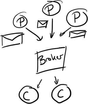
Kafka’s model is pretty general; messages are published onto topics by producers, stored on disk and made available to consumers. It’s important to note that messages are pulled by consumers to avoid needing any complex throttling in the event of slow consumption.

Kafka doesn’t dictate any serialisation it just expects a payload of byte[]. We’re using Protocol Buffers for most of our topics to make it easier to evolve schemas over time. Having a repository of definitions has also made it slightly easier for teams to see what events they can publish and what they can consume.

This is what it looks like in Clojure code using clj-kafka.

We use messages to record the products that are shown across our site, the searches that people perform, emails that are sent (and bounced), web requests and more. In total it’s probably a few million messages a day.

Metadata and State

Kafka uses Zookeeper for various bits of meta-information, including tracking which messages have already been retrieved by a consumer. To that end, it is the consumers responsibility to track consumption- not the broker. Kafka’s client library already contains a Zookeeper consumer that will track the message offsets that have been consumed.

As an side, the broker keeps no state about any of the consumers directly. This keeps it simple and means that there’s no need for complex structures kept in memory reducing the need for garbage collections.

When messages are received they are written to a log file (well, handed off to the OS to write) named after the topic; these are serial append files so individual writes don’t need to block or interfere with each other.

When reading messages consumers simply access the file and read data from it. It’s possible to perform parallel consumption through partitioned topics although this isn’t something we’ve needed yet.

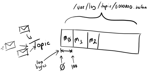
Messages are tracked by their offset- letting consumers access from a given point into the topic. A consumer can connect and ask for all messages that Kafka has stored currently, or from a specified offset. This relatively long retention (compared to other messaging systems) makes Kafka extremely useful to support both real-time and batch reads. Further, because it takes advantage of disk throughput it makes it a cost-effective system too.

The broker can be configured to keep messages up to a specified quantity or for a set period of time. Our broker is configured to keep messages for up to 20 days, after that and you’ll need to go elsehwere (most topics are stored on HDFS afterwards). This characteristic that has made it so useful for us- it makes getting data out of applications and servers and into other systems much easier, and more reliable, than periodically aggregating log files.

Performance

Kafka’s performance (and the design that achieves it) is derived from the observation that disk throughput has outpaced latency; it writes and reads sequentially and uses the operating system’s file system caches rather than trying to maintain its own- minimising the JVM working set, and again, avoiding garbage collections.

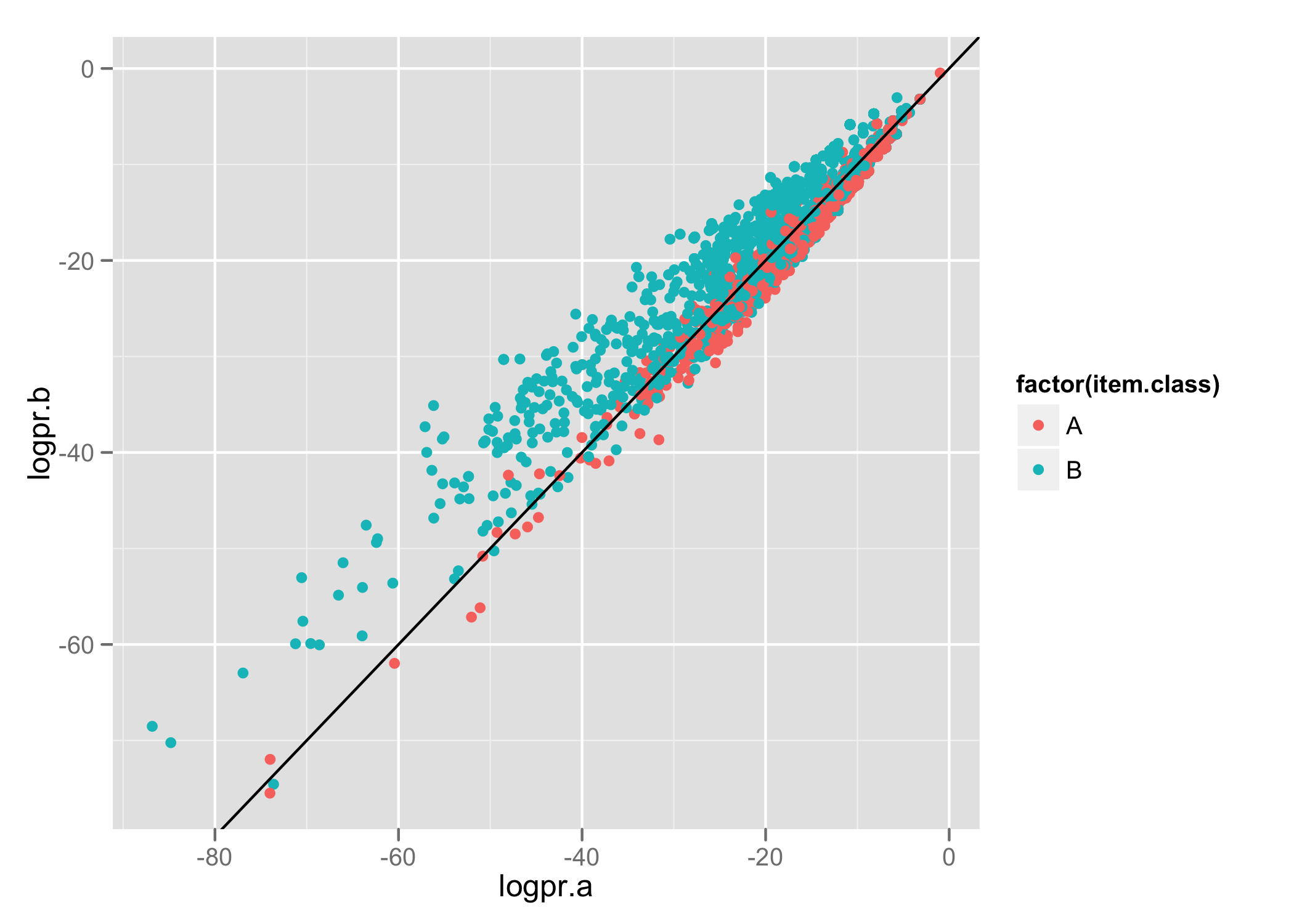
The plot below shows results published within an ACM article; their experiment was to measure how quickly they could read 4-byte values sequentially and randomly from different storage.

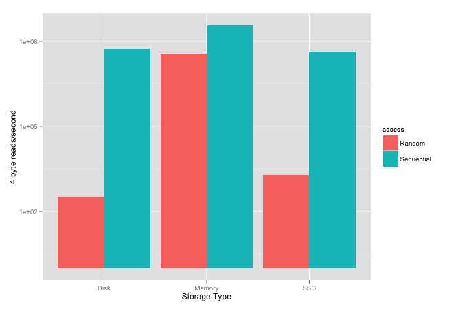
Please note the scale is logarithmic because the difference between random and sequential is so large for both SSD and spinning disks.

Interestingly, it shows that sequential disk access, spinning or SSD, is faster than random memory access. It also shows that, in their tests, sequential spinning disk performance was higher than SSD.

In short, using sequential reads lets Kafka get performance close to random memory access. And, by keeping very little in the way of metadata, the broker can be extremely lightweight.

If anyone is interested, the Kafka design document is very interesting and accessible.

Batch Load into HDFS

As I mentioned earlier, most topics are stored on HDFS so that we can maximise the amount of analysis we can perform over time.

We use a Hadoop job that is derived from the code included within the Kafka distribution.

The process looks a little like this:

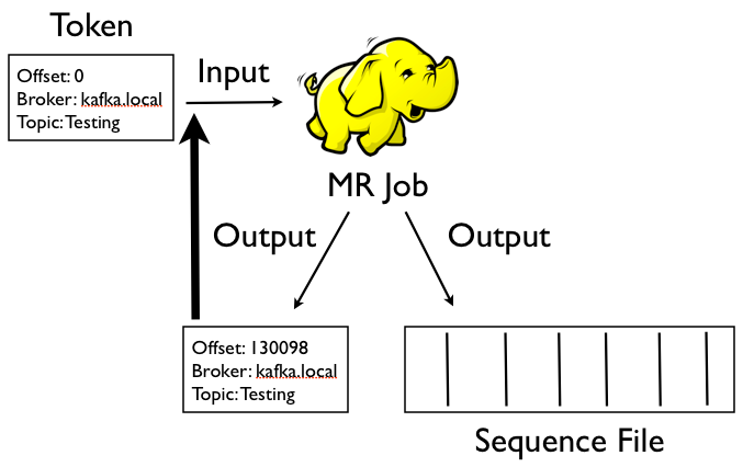
Each topic has a directory on HDFS that contains 2 further subtrees: these contain offset token files and data files. The input to the Hadoop job is an offset token file which contains the details of the broker to consume from, the message offset to read from, and the name of the topic. Although it’s a SequenceFile the value bytes contain a string that looks like this:

broker.host.com topic-name  102991

The job uses a RecordReader that connects to the Kafka broker and passes the message payload directly through to the mapper. Most of the time the mapper will just write the whole message bytes directly out which is then written using Hadoop’s SequenceFileOutputFormat (so we can compress and split the data for higher-volume topics) and Hadoop’s MultipleOutputs so we can write out 2 files- the data file and a newly updated offset token file.

For example, if we run the job and consume from offset 102991 to offset 918280, this will be written to the offset token file:

broker.host.com topic-name  918280

Note that the contents of the file is exactly the same as before just with the offset updated. All the state necessary to perform incremental loads is managed by the offset token files.

This ensures that the next time the job runs we can incrementally load only the new messages. If we introduce a bug into the Hadoop load job we can just delete one or more of the token files to cause the job to load from further back in time.

Again, Kafka’s inherent persistence makes dealing with these kinds of HDFS loads much easier than dealing with polling for logs. Previously we’d used other databases to store metadata about the daily rotated logs we’d pulled but there was lots of additional computation in splitting apart files that would span days- incremental loads with Kafka are infinitely cleaner and efficient.

Kafka has helped us both simplify our data collection infrastructure, letting us evolve and grow it more flexibly, and provided the basis for building real-time systems. It’s extremely simple and very easy to setup and configure, I’d highly recommend it for anyone playing in a similar space.

Related Stuff

As I publish this LinkedIn have just announced the release of Camus: their Kafka to HDFS pipeline. The pipeline I’ve described above was inspired by the early Hadoop support within Kafka but has since evolved into something specific for use at uSwitch.

Twitter also just published about their use of Kafka and Storm to provide real-time search.

I can also recommend reading “The Unified Logging Infrastructure for Data Analytics at Twitter” paper that was published late last year.

Finally, this post was based on a brief presentation I gave internally in May last year: Kafka a Little Introduction

Clojure - From Callbacks to Sequences

2012-12-19T15:35:00Z

I was doing some work with a colleague earlier this week which involved connecting to an internal RabbitMQ broker and transforming some messages before forwarding them to our Kafka broker.

We’re using langohr to connect to RabbitMQ. Its consumer and queue documentation shows how to use the subscribe function to connect to a broker and print messages that arrive:

The example above is pretty close to what we started working with earlier today. It’s also quite similar to a lot of other code I’ve written in the past: connect to a broker or service and provide a block/function to be called when something interesting happens.

Sequences, not handlers

Although there’s nothing wrong with this I think there’s a nicer way: flip the responsibility so instead of the subscriber pushing to our handler function we consume it through Clojure’s sequence abstraction.

This is the approach I took when I wrote clj-kafka, a Clojure library to interact with LinkedIn’s Kafka (as an aside, Kafka is really cool- I’m planning a blog post on how we’ve been building a new data platform for uSwitch.com but it’s well worth checking out).

Here’s a little example of consuming messages through a sequence that’s taken from the clj-kafka README:

We create our consumer and access messages through a sequence abstraction by calling messages with the topic we wish to consume from.

The advantage of exposing the items through a sequence is that it becomes instantly composable with the many functions that already exist within Clojure: map, filter, remove etc.

In my experience, when writing consumption code that uses handler functions/callbacks I’ve ended up with code that looks like this:

It makes consuming data more complicated and pulls more complexity into the handler function than necessary.

Push to Pull

This is all made possible thanks to a lovely function written by Christophe Grande:

The function returns a vector containing 2 important parts: the sequence, and a function to put things into that sequence.

Returning to our original RabbitMQ example, we can change the subscriber code to use pipe to return the sequence that accesses the queue of messages:

We can then map, filter and more.

We pull responsibility out of the handler function and into the consumption of the sequence. This is really important, and it compliments something else which I’ve recently noticed myself doing more often.

In the handler function above I convert the function parameters to a map containing :payload, :ch and :msg-meta. In our actual application we’re only concerned with reading the message payload and converting it from a JSON string to a Clojure map.

Initially, we started writing something similar to this:

We have a function that exposes the messages through a sequence, but we pass a kind of transformation function as the last argument to subscriber-seq. This initially felt ok: subscriber-seq calls our handler and extracts the payload into our desired representation before putting it into the queue that backs the sequence.

But we’re pushing more responsibility into subscriber-seq than needs to be there.

We’re just extracting and transforming messages as they appear in the sequence so we can and should be building upon Clojure's existing functions: map and the like. The code below feels much better:

It feels better for a similar reason as moving the handler to a sequence- we’re making our function less complex and encouraging the composition through the many functions that already exist. Line 13 is a great example of this for me- map’ing a composite function to transform the incoming data rather than adding more work into subscriber-seq.

Pipe

I’ve probably used Christophe’s pipe function 3 or 4 times this year to take code that started with handler functions and evolved it to deal with sequences. I think it’s a really neat way of making callback-based APIs more elegant.

Multi-armed Bandit Optimisation in Clojure

2012-12-17T13:47:00Z

The multi-armed (also often referred to as K-armed) bandit problem models the problem a gambler faces when attempting maximise the reward from playing multiple machines with varying rewards.

For example, let’s assume you are standing in front of 3 arms and that you don’t know the rate at which they will reward you. How do you set about the task of pulling the arms to maximise your cumulative reward?

It turns out there’s a fair bit of literature on this topic, and it’s also the subject of a recent O’Reilly book: “Bandit Algorithms for Website Optimization” by John Myles White (who also co-wrote the excellent Machine Learning for Hackers).

This article discusses my implementation of the algorithms which is available on GitHub and Clojars: https://github.com/pingles/clj-bandit.

Enter Clojure

I was happy to attend this year’s clojure-conj and started reading through the PDF whilst on the flight out. Over the next few evenings, afternoons and mornings (whenever I could squeeze in time) I spent some time hacking away at implementing the algorithms in Clojure. It was great fun and I pushed the results into a library: clj-bandit.

I was initially keen on implementing the same algorithms and being able to reproduce the results shown in the book. Since then I’ve spent a little time tweaking parts of the code to be a bit more functional/idiomatic. The bulk of this post covers this transition.

I started with a structure that looked like this:

From there I started layering on functions that select the arm with each algorithm’s select-arm implemented in its own namespace.

One of the simplest algorithms is Epsilon-Greedy: it applies a fixed probability when deciding whether to explore (try other arms) or exploit (pull the currently highest-rewarding arm).

The code, as implemented in clj-bandit, looks like this:

We generate a random number (between 0 and 1) and either pick the best performing or a random item from the arms.

In my initial implementation I kept algorithm functions together in a protocol, and used another protocol for storing/retrieving arm data. These were reified into an ‘algorithm’:

Applying select-arm to the current arm state would select the next arm to pull. Having pulled the arm, update-reward would let the ‘player’ track whether they were rewarded or not.

This worked, but it looked a little kludgey and made the corresponding monte-carlo simulation code equivalently disgusting.

I initially wanted to implement all the algorithms so I could reproduce the same results that were included in the book but the resulting code definitely didn’t feel right.

More Functional

After returning from the conference I started looking at the code and started moving a few functions around. I dropped the protocols and went back to the original datastructure to hold the algorithm’s current view of the world.

I decided to change my approach slightly and introduced a record to hold data about the arm.

The algorithms don’t need to know about the identity of any individual arm- they just need to pick one from the set. It tidied a lot of the code in the algorithms. For example, here’s the select-arm code from the UCB algorithm:

Functional Simulation

The cool part about the book and it’s accompanying code is that includes a simulation suitable for measuring the performance and behaviour of each of the algorithms.

This is important because the bandit algorithms have a complex feedback cycle: their behaviour is constantly changing in the light of data given to them during their lifetime.

For example, following from the code by John Myles White in his book, we can visualise the algorithm’s performance over time. One measure is accuracy (that is, how likely is the algorithm to pick the highest paying arm at a given iteration) and we can see the performance across algorithms over time, and according to their exploration/exploitation parameters, in the plot below:

The simulation works by using a series of simulated bandit arms. These will reward randomly according to a specified probability:

We can model the problem neatly by creating a function representing the arm, we can then pull the arm by applying the function.

As I mentioned earlier, when the code included protocols for algorithms and storage, the simulation code ended up being pretty messy. After I’d dropped those everything felt a little cleaner and more Clojure-y. This felt more apparent when it came to rewriting the simulation harness.

clj-bandit.simulate has all the code, but the key part was the introduction of 2 functions that performed the simulation:

simulation-seq creates a sequence through iterate’ing the simulate function. simulate is passed a map that contains the current state of the algorithm (the performance of the arms), it returns the updated state (based on the pull during that iteration) and tracks the cumulative reward. Given we’re most interested in the performance of the algorithm we can then just (map :result ...) across the sequence. Much nicer than nested doseq’s!

Further Work

At uSwitch we’re interested in experimenting with multi-armed bandit algorithms. We can use simulation to estimate performance using already observed data. But, we’d also need to do a little work to consume these algorithms into web applications.

There are existing Clojure libraries for embedding optimisations into your Ring application:

These both provide implementations of the algorithms and for storing their state in stores like Redis.

I chose to work through the book because I was interested in learning more about the algorithms but I also like the idea of keeping the algorithms and application concerns separate.

Because of that I’m keen to work on a separate library that makes consuming the algorithms from clj-bandit into a Ring application easier. I’m hoping that over the coming holiday season I’ll get a chance to spend a few more hours working on it.

Analysing and predicting performance of our Neo4j Cascading Connector with linear regression in R

2012-11-22T13:51:00Z

As I mentioned in an earlier article, Paul and I have produced a library to help connect Cascading and Neo4j making it easy to sink data from Hadoop with Cascading flows into a Neo4j instance. Whilst we were waiting for our jobs to run we had a little fun with some regression analysis to optimise the performance. This post covers how we did it with R.

I’m posting because it wasn’t something I’d done before and it turned out to be pretty good fun. We played with it for a day and haven’t done much else with it since so I’m also publishing in case it’s useful for others.

We improved the write performance of our library by adding support for batching- collecting mutations into sets of transactions that are batched through Neo4j’s REST API. This improved performance (rather than using a request/response for every mutation) but also meant we needed to specify a chunk size; writing all mutations in a single transaction would be impossible.

There are 2 indepent variables that we could affect to tweak performance: the batch size and the number of simultaneous connections that are making those batch calls. N.B this assumes any other hidden factors remain constant.

For us, running this on a Hadoop cluster, these 2 variables determine the batch size in combination with the number of Hadoop’s reduce or map tasks concurrently executing.

We took some measurements during a few runs of the connector across our production data to help understand whether we were making the library faster. We then produced a regression model from the data and use the optimize function to help identify the sweet spot for our job’s performance.

We had 7 runs on our production Hadoop cluster. We let the reduce tasks (where the Neo4j write operations were occurring) run across genuine data for 5 minutes and measured how many nodes were successfully added to our Neo4j server. Although the cluster was under capacity (so the time wouldn’t include any idling/waiting) our Neo4j server instance runs on some internal virtualised infrastructure and so could have exhibited variance beyond our changes.

The results for our 7 observerations are in the table below:

Test No.	Number of Reducers	Batch Size	Nodes per minute
1	1	10	5304.4
2	4	10	13218.8
3	4	20	13265.636
4	8	5	11289.2
5	8	10	17682.2
6	16	10	20984.2
7	8	20	20201.6

Regression in R

A regression lets us attempt to predict the value of a continuous variable based upon the value of one or more other independent variables. It also lets us quantify the strength of the relationship between the dependent variable and independent variables.

Given our experiment, we could determine whether batch size and the number of reducers (the independent variables) affected the number of Neo4j nodes we could create per minute (the dependent variable). If there was, we would use values for those 2 variables to predict performance.

The first stage is to load the experiment data into R and get it into a data frame. Once we’ve loaded it we can use R’s lm function to fit a linear model and look at our data.

In the above, the formula parameter to lm lets us describe that nodes.per.minute is our dependent variable (our outcome), and reducers and batch.size are our independent variables (our predictors).

Much like other analysis in R, the first thing we can look at is a summary of this model, which produces the following:

lm(formula = nodes.per.minute ~ reducers + batch.size, data = results)

Residuals:
    1     2     3     4     5     6     7 
-2330  2591 -1756 -1135  3062 -1621  1188 

Coefficients:
            Estimate Std. Error t value Pr(>|t|)  
(Intercept)   2242.8     3296.7   0.680   0.5336  
reducers       998.1      235.6   4.236   0.0133 *
batch.size     439.3      199.3   2.204   0.0922 .
---
Signif. codes:  0 ‘***’ 0.001 ‘**’ 0.01 ‘*’ 0.05 ‘.’ 0.1 ‘ ’ 1 

Residual standard error: 2735 on 4 degrees of freedom
Multiple R-squared: 0.8362, Adjusted R-squared: 0.7543 
F-statistic: 10.21 on 2 and 4 DF,  p-value: 0.02683

The summary data tells us that the model supports the data relatively well. Our R-squared is 0.075 and both batch size and reducer size are considered significant.

But, what if we tweak our model? We suspect that the shape of the performance through increasing reducers and batch size is unlikely to exhibit linear growth. We can change the formula of our model and see whether we can improve the accuracy of our model:

And let’s the the results of calling summary(model):

Call:
lm(formula = nodes.per.minute ~ reducers + I(reducers^2) + batch.size + 
    I(batch.size^2), data = results)

Residuals:
         1          2          3          4          5          6          7 
-2.433e+02  9.318e+02 -3.995e+02  9.663e-13 -7.417e+02  5.323e+01  3.995e+02 

Coefficients:
                 Estimate Std. Error t value Pr(>|t|)  
(Intercept)     -15672.16    3821.48  -4.101   0.0546 .
reducers          2755.10     337.07   8.174   0.0146 *
I(reducers^2)     -101.74      18.95  -5.370   0.0330 *
batch.size        2716.07     540.07   5.029   0.0373 *
I(batch.size^2)    -85.94      19.91  -4.316   0.0497 *
---
Signif. codes:  0 ‘***’ 0.001 ‘**’ 0.01 ‘*’ 0.05 ‘.’ 0.1 ‘ ’ 1 

Residual standard error: 948.6 on 2 degrees of freedom
Multiple R-squared: 0.9901, Adjusted R-squared: 0.9704 
F-statistic: 50.25 on 4 and 2 DF,  p-value: 0.01961

Our R-squared is now 0.9704- our second model fits the data better than our first model.

Optimization

Given the above, we’d like to understand the values for batch size and number of reducers that will give us the highest throughput.

R has an optimize function that, given a range of values for a function parameter, returns the optimal argument for the return value.

We can create a function that calls predict.lm with our model to predict values. We can then use the optimize function to find our optimal solution:

We use a set batch size of 20 and optimize to discover that the optimal number of reducers is 13 with a throughput of 22,924 nodes/minute. The second command optimizes for batch size with a fixed number of reducers. Again, it suggests a batch size of 15 for an overall throughput of 24,409 nodes/minute.

This supports what we observed earlier with the summary data: number of reducers is more significant than batch size for predicting throughput.

I’m extremely new to most of R (and statistics too if I’m honest- the last year is the most I’ve done since university) so if anyone could tell me if there’s a way to perform an optimization for both variables that would be awesome.

Please note this post was more about our experimentation and the process- I suspect our data might be prone to systematic error and problems because we only have a few observations. I’d love to run more experiments and get more measurements but we moved on to a new problem :)

Sinking Data to Neo4j from Hadoop with Cascading

2012-11-22T10:53:00Z

Recently, I worked with a colleague (Paul Lam, aka @Quantisan on building a connector library to let Cascading interoperate with Neo4j: cascading.neo4j. Paul had been experimenting with Neo4j and Cypher to explore our data through graphs and we wanted an easy way to flow our existing data on Hadoop into Neo4j.

The data processing pipeline we’ve been growing at uSwitch.com is built around Cascalog, Hive, Hadoop and Kafka.

Once the data has been aggregated and stored a lot of our ETL is performed upon Cascalog and, by extension, Cascading. Querying/analysis is a mix of Cascalog and Hive. This layer is built upon our long-term data storage system: Hadoop; this, all combined, lets us store high-resolution data immutably at a much lower cost than uSwitch’s previous platform.

Cascading is:

application framework for Java developers to quickly and easily develop robust Data Analytics and Data Management applications on Apache Hadoop

Cascading provides a model on top of Hadoop’s very file-oriented, raw MapReduce API. It models the world around flows of data (Tuples), between Taps and according to Schemes.

For example, in Hadoop you might configure a job that reads data from a SequenceFile at a given location on HDFS. Cascading separates the 2 into slightly different concerns- the Tap would represent file storage on HDFS, the Scheme would be configured to read data according to the SequenceFile format.

Cascading provides a lot of classes to make it easier to build flows that join and aggregate data without you needing to write lots of boiler-plate MapReduce code.

Here’s an example of writing a Cascading flow (taken from the README of our cascading.neo4j library). It reads data from a delimited file (representing the Neo4j Nodes we want to create), and flows every record to our Neo4j Tap.

Although we use Cascading, really the majority of that is through Cascalog- a Clojure library that provides a datalog like language for analysing our data.

We wrote a small test flow we could use whilst testing our connector, a similar Cascalog example for the Cascading code above looks like this:

Our library, cascading.neo4j (hosted on Conjars.org) provides a Tap and Scheme suitable for sinking (writing data) to a Neo4j server using their REST connector. We extend and implement Cascading classes and interfaces making it easy to then integrate into our Cascalog processing.

cascading.neo4j allows you to create nodes, set properties on those node, add nodes to an exact match index, and create relationships (again with properties) between those nodes.

I should point out that cascading.neo4j may not be suitable for all batch processing purposes: most significantly, its pretty slow. Our production Neo4j server (on our internal virtualised infrastructure) lets us sink around 20,000 nodes per minute through the REST api. This is certainly a lot slower than Neo4j’s Batch Insert API and may make it unusable in some situations.

However, if the connector is fast enough for you it means you can sink data directly to Neo4j from your existing Cascading flows.

Performance

Whilst tweaking and tuning the connector we ran through Neo4j’s Linux Performance Guide (a great piece of technical documentation) that helped us boost performance a fair bit.

We also noticed the REST library allows for transactions to hold batch operations- to include multiple mutations in the same roundtrip. Our Neo4j RecordWriter will chunk batches- rather than writing all records in one go, you can specify the size.

We ran some tests and, on our infrastructure, using batch sizes of around 15 and 13 reducers (that is 13 ‘connections’ to our Neo4j REST api) yield the best performance of around 20,000 nodes per minute. We collected some numbers and Paul suggested we could have some fun putting those through a regression which will be the subject of my next post :)

Next steps

It’s currently still evolving a little and there’s a bit of duplicate code between the Hadoop and Local sections of the code. The biggest restrictions are it currently only supports sinking (writing) data and it’s speed may make it unsuitable for flowing very large graphs.

Hopefully this will be useful for some people and Paul and I would love pull requests for our little project.

Compressing CloudFront Assets and dfl8.co

2012-08-18T13:44:00Z

Amazon’s web services have made rebuilding uSwitch.com so much easier. We’re gradually moving more and more static assets to CloudFront (although most visitors are in the UK responses have much lower latencies than direct from S3 or even our own nginx servers). CloudFront doesn't support serving gzip'ed content direct from S3 out of the box.

Because of this, up until last week we were serving uncompressed assets, at least anything that wasn’t already compressed (such as images). Last week we put together a simple static assets nginx server to help compress things.

Whilst doing the work for uSwitch.com I realised it would be trivial to write an application that would let any CloudFront user compress to any S3 bucket by using an equivalent URL structure. So I knocked up a quick node.js app that’s hosted on Heroku for all to use: dfl8.co.

dfl8.co

S3 assets can be referenced through a pretty simple URL structure. By creating an app that behaves in the same way, and proxies (whilst compressing) the response, it would be easy to create a compressible S3 for everyone.

For example, the URL http://pingles-example.s3.amazonaws.com/sample.css references the S3 bucket pingles-example and the object we want to retrieve is identified by the name /sample.css.

The same resource can be accessed through http://pingles-example.dfl8.co/sample.css and will be gzip compressed. CloudFront now lets you specify custom origins so for the above you’d add http://pingles-example.dfl8.co to setup a CloudFront distribution for the pingles-example S3 bucket.

At the moment it will only proxy public resources. Response latency also seems quite high at the moment but given the aim is to get content into the highly-cached and optimised CloudFront I’m not too fussed by it.

Evaluating classifier results with R part 2

2012-07-15T21:06:00Z

In a previous article I showed how to visualise the results of a classifier using ggplot2 in R. In the same article I mentioned that Alex, a colleague at Forward, had suggested looking further at R’s caret package that would produce more detailed statistics about the overall performance of the classifer and within individual classes.

Confusion Matrix

Using ggplot2 we can produce a plot like the one below: a visual representation of a confusion matrix. It gives us a nice overview but doesn’t reveal much about the specific performance characteristics of our classifier.

To produce our measures, we run our classifier across a set of test data and capture both the actual class and the predicted class. Our results are stored in a CSV file and will look a little like this:

actual, predicted
A, B
B, B,
C, C
B, A

Analysing with Caret

With our results data as above we can run the following to produce a confusion matrix with caret:

results.matrix now contains a confusionMatrix full of information. Let’s take a look at some of what it shows. The first table shows the contents of our matrix:

Reference
Prediction              A     B     C     D
A                     211   3     1     0
B                     9     26756 6     17
C                     1     12    1166  1
D                     0     18    3     1318

Each column holds the reference (or actual) data and within each row is the prediction. The diagonal represents instances where our observation correctly predicted the class of the item.

The next section contains summary statistics for the results:

Overall Statistics

                     Accuracy : 0.9107          
                       95% CI : (0.9083, 0.9131)
          No Information Rate : 0.5306          
          P-Value [Acc > NIR] : < 2.2e-16

Overall accuracy is calculated at just over 90% with a p-value of 2 x 10^-16, or 0.00000000000000022. Our classifier seems to be doing a pretty reasonable job of classifying items.

Our classifier is being tested by putting items into 1 of 13 categories- caret also produces a final section of statistics for the performance of each class.

Class: A        Class: B  ...   Class: J
Sensitivity             0.761733        0.9478          0.456693
Specificity             0.998961        0.9748          0.999962
Pos Pred Value          0.793233        0.9770          0.966667 
Neg Pred Value          0.998753        0.9429          0.998702
Prevalence              0.005206        0.5306          0.002387
Detection Rate          0.003966        0.5029          0.001090
Detection Prevalence    0.005000        0.5147          0.001128

The above shows some really interesting data.

Sensitivity and specificity respectively help us measure the performance of the classifier in correctly predicting the actual class of an item and not predicting the class of an item that is of a different class; it measures true positive and true negative performance.

From the above data we can see that our classifier correctly identified class B 94.78% of the time. That is, when we should have predicted class B we did. Further, when we shouldn’t have predicted class B we didn’t for 97.48% of examples. We can contrast this to class J: our specificity (true negative) is over 99% but our sensitivity (true positive) is around 45%; we do a poor job of positively identifying items of this class.

Caret has also calculated a prevalence measure- that is, of all observations, how many were of items that actually belonged to the specified class; it calculates the prevalence of a class within a population.

Using the previously defined sensitivity and specificity, and prevalance measures caret can calculate Positive predictive value and Negative predictive value. These are important as they reflect the probability that a true positive/true negative is correct given knowledge about the prevalence of classes within the population. Class J has a positive predictive value of over 96%: despite our classifier only being able to positively identify objects 45% of the time there’s a 96% chance that, when it does, such a classification is correct.

The caret documentation has some references to relevant papers discussing the measures it calculates.

Visualising classifier results with R and ggplot2

2012-07-14T15:13:00Z

Earlier in the year, myself and some colleagues started working on building better data processing tools for uSwitch.com. Part of the theory/reflection of this is captured in a presentation I was privileged to give at EuroClojure (titled Users as Data).

In the last few days, our data team (Thibaut, Paul and I) have been playing around with some of the data we collect and using it to build some classifiers. Precision and Recall provide quantitative measures but reading through Machine Learning for Hackers showed some nice ways to visualise results.

Binary Classifier

Our first classifier attempted to classify data into 2 groups. Using R and ggplot2 I produced a plot (similar to the one presented in the Machine Learning for Hackers book) to show the results of the classifier.

Our results were captured in a CSV file and looked a little like this:

A,0.25,0.15
A,0.2,0.19
B,0.19,0.25

Each line contains the item's actual class, the predicted probability for membership of class A, and the predicted probability for membership of class B. Using ggplot2 we produce the following:

Items have been classified into 2 groups- A and B. The axis show the log probability (we’re using Naive Bayes to classify items) that the item belongs to the specified class. We use colour to identify the actual class for items and draw a line to represent the decision boundary (i.e. which of the 2 classes did our model predict).

This lets us nicely see the relationship between predicted and actual classes.

We can see there’s a bit of an overlap down the decision boundary line and we’re able to do a better job for classifying items in category B than A.

The R code to produce the plot above is as follows. Note that because we had many millions of observations I randomly sampled to make it possible to compute on my laptop :)

More Classes!

But what if we want to see compare the results when we’re classifying items into more than 1 group?

After chatting to Alex Farquhar (another data guy at Forward) he suggested plotting a confusion matrix.

Below shows the plot we produced that compares the actual and predicted classes for 14 items.

The y-axis shows the predicted class for all items, and the x-axis shows the actual class. The tiles are coloured according to the frequency of the intersection of the two classes thus the diagonal represents where we predict the actual class. The colour represents the relative frequency of that observation in our data; given some classes occur more frequently we normalize the values before plotting.

Any row of tiles (save for the diagonal) represents instances where we falsely identified items as belonging to the specified class. In the rendered plot we can see that items in Class G were often identified for items belonging to all other classes.

Our input data looked a little like this:

1,0,0
0,3,0
1,0,2

It’s a direct encoding of our matrix- each column represents data for classes A to N, and each row represents data for classes A to N. The diagonal holds data for A,A, B,B, etc.

The R code to plot the confusion matrix is as follows:

Alex also suggested using the caret package which includes a function to build the confusion matrix from observations directly and also provides some useful summary statistics. I’m going to hack on our classifier’s Clojure code a little more and will be sure to post again with the findings!

Protocol Buffers with Clojure and Leiningen

2012-01-20T10:08:00Z

This week I’ve been prototyping some data processing tools that will work across the platforms we use (Ruby, Clojure, .NET). Having not tried Protocol Buffers before I thought I’d spike it out and see how it might fit.

Protocol Buffers

The Google page obviously has a lot more detail but for anyone who’s not seen them: you define your messages in an intermediate language before compiling into your target language.

There’s a Ruby library that makes it trivially easy to generate Ruby code so you can create messages as follows:

Clojure and Leiningen

The next step was to see how these messages would interact with Clojure and Java. Fortunately, there’s already a few options and I tried out clojure-protobuf which conveniently includes a Leiningen task for running both the Protocol Buffer compiler protoc and javac.

I added the dependency to my project.clj:

[protobuf "0.6.0-beta2"]

At the time, the protobuf library expected your .proto files to be placed in a ./proto directory under your project root. I forked to add a :proto-path so that I could pull in the files from a git submodule.

Assuming you have a proto file or two in your proto source directory, you should be able to invoke the compiler by running

$ lein protobuf compile
Compiling person.proto to /Users/paul/Work/forward/data-spike/protosrc
Compiling 1 source files to /Users/paul/Work/forward/data-spike/classes

You should now see some Java .class files in your ./classes directory.

Using clojure-protobuf to load an object from a byte array looks as follows:

Uberjar Time

I ran into a little trouble when I came to build the command-line tool and deploy it. When building with lein uberjar it seemed that the ./classes directory was being cleaned causing the protobuf compiled Java classes to be unavailable to the application (causing the rest of the application to fail to build- I was using tools.cli with a main fn which meant using :gen-class).

I always turn to Leiningen’s sample project.clj and saw :clean-non-project-classes. The comment mentioned it was set to false by default so that wasn’t it.

It turns out that Leiningen’s uberjar task checks a different option when determining whether to clean the project before executing: :disable-implicit-clean. I added :disable-implicit-clean true to our project.clj and all was good:

$ lein protobuf compile, uberjar

I wasn’t a registered user of the Leiningen mailing list (and am waiting for my question to be moderated) but it feels like uberjar should honour :clean-non-project-class too. I’d love to submit a patch to earn myself a sticker :)